
This post is a continuation of the preceding post on (a,b,0) class. This post introduces the class of discrete discrete distributions called the (a,b,1) class.
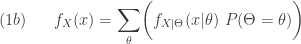
The discussion in this post has a great deal of technical details. A concise summary of the (a,b,0) class and (a,b,1) class is found here.
The (a,b,1) Class
A counting distribution is a discrete probability distribution that takes on the non-negative integers. Let 

![P_k=P[N=k]](https://s0.wp.com/latex.php?latex=P_k%3DP%5BN%3Dk%5D&bg=ffffff&fg=333333&s=0&c=20201002)


(1)……….

For a member of the (a,b,0) class, the initial probability 

(2)……….
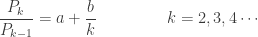
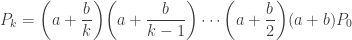
The recursion in the (a,b,1) class begins at 


There are two subclasses in the (a,b,1) class of distributions. They are determined by whether 

This is how we will proceed. Using a given distribution in the (a,b,0) class as a starting point, we show how to derive the zero-truncated distribution. From a given zero-truncated distribution, we show how to derive the zero-modified distribution.
The name of the (a,b,1) distribution has the same (a,b,0) name with either zero-truncated or zero-modified as the prefix. For example, if the starting point is the negative binomial distribution in the (a,b,0) class, then the derived distributions in the (a.b.1) class are the zero-truncated negative binomial distribution and the zero-modified negative binomial distribution.
There are only three distributions in the (a,b,0) class – Poisson, binomial and negative binomial. Then the (a,b,1) class contains the zero-truncated and zero-modified versions of these three distributions. However, the (a,b,1) class contained distributions that are not modifications of the (a,b,0) distributions. We discuss three such additional distributions – extended truncated negative binomial (ETNB) distribution, logarithmic distribution and Sibuya distribution. These three distributions that are not derived from an (a,b,0) distribution are discussed in a separate section below.
We present three examples demonstrating how using a base (a,b,0) negative binomial distribution to derive a zero-truncated negative binomial distribution (Example 1) and a zero-modified negative binomial distribution (Example 2). We also give an example for ETNB distribution (Example 3).
Notations
To facilitate discussion, let’s fix some notations. To clearly denote the distributions, notations without superscripts and subscripts refer to the (a,b,0) distributions. Notations with the superscript T (or subscript T) refer to the zero-truncated distributions in the (a,b,1) class. Likewise notations with the superscript M (or subscript M) refer to the zero-modified distributions in the (a,b,1) class.
For example, the following are the probability function (pf) and the probability generating function (pgf) of a distribution from the (a,b,0) class.
(3)……….
![\displaystyle \begin{aligned}&P_k=P[N=k] \\&P(z)=\sum \limits_{k=0}^\infty P_k z^k \end{aligned}](https://s0.wp.com/latex.php?latex=%5Cdisplaystyle+%5Cbegin%7Baligned%7D%26P_k%3DP%5BN%3Dk%5D+%5C%5C%26P%28z%29%3D%5Csum+%5Climits_%7Bk%3D0%7D%5E%5Cinfty+P_k+z%5Ek++%5Cend%7Baligned%7D&bg=ffffff&fg=333333&s=0&c=20201002)
The following shows the notations for the pf and pgf for a zero-truncated distribution from the (a,b,1) class.
(4)……….
![\displaystyle \begin{aligned}&P_k^T=P[N_T=k] \\&P^T(z)=\sum \limits_{k=1}^\infty P_k^T z^k \end{aligned}](https://s0.wp.com/latex.php?latex=%5Cdisplaystyle+%5Cbegin%7Baligned%7D%26P_k%5ET%3DP%5BN_T%3Dk%5D+%5C%5C%26P%5ET%28z%29%3D%5Csum+%5Climits_%7Bk%3D1%7D%5E%5Cinfty+P_k%5ET+z%5Ek++%5Cend%7Baligned%7D&bg=ffffff&fg=333333&s=0&c=20201002)
The following shows the notations for the pf and pgf for a zero-modified distribution from the (a,b,1) class.
(5)……….
![\displaystyle \begin{aligned}&P_k^M=P[N_M=k] \\&P^M(z)=\sum \limits_{k=0}^\infty P_k^M z^k \end{aligned}](https://s0.wp.com/latex.php?latex=%5Cdisplaystyle+%5Cbegin%7Baligned%7D%26P_k%5EM%3DP%5BN_M%3Dk%5D+%5C%5C%26P%5EM%28z%29%3D%5Csum+%5Climits_%7Bk%3D0%7D%5E%5Cinfty+P_k%5EM+z%5Ek++%5Cend%7Baligned%7D&bg=ffffff&fg=333333&s=0&c=20201002)
Whenever it is convenient to do so, 

Zero-Truncated Distributions
The focus in this section is on the zero-truncated distributions that originate from the (a,b,0) class. The three distributions indicated above (ETNB, logarithmic and Shibuya) are discussed in a separate section below.
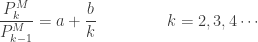
Suppose we start with a distribution from the (a,b,0) class, with the notations 
(6)……….

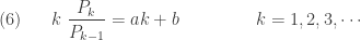
The recursion relation (6) is identical to the one in (2). The recursion begins at
(7)……….

The probabilities 


(8)……….
![\displaystyle P^T(z)=\sum \limits_{k=1}^\infty P_k^T \ z^k =\frac{1}{1-P_0} \ [P(z)-P_0]](https://s0.wp.com/latex.php?latex=%5Cdisplaystyle+P%5ET%28z%29%3D%5Csum+%5Climits_%7Bk%3D1%7D%5E%5Cinfty+P_k%5ET+%5C+z%5Ek+%3D%5Cfrac%7B1%7D%7B1-P_0%7D+%5C+%5BP%28z%29-P_0%5D+&bg=ffffff&fg=333333&s=0&c=20201002)
(9)……….
![\displaystyle E[N_T]=\frac{1}{1-P_0} \ E[N]](https://s0.wp.com/latex.php?latex=%5Cdisplaystyle+E%5BN_T%5D%3D%5Cfrac%7B1%7D%7B1-P_0%7D+%5C+E%5BN%5D+&bg=ffffff&fg=333333&s=0&c=20201002)
(10)……..
![\displaystyle E[N_T^2]=\frac{1}{1-P_0} \ E[N^2]](https://s0.wp.com/latex.php?latex=%5Cdisplaystyle+E%5BN_T%5E2%5D%3D%5Cfrac%7B1%7D%7B1-P_0%7D+%5C+E%5BN%5E2%5D+&bg=ffffff&fg=333333&s=0&c=20201002)
(11)……..
![\displaystyle \begin{aligned} Var[N_T]&=\frac{1}{1-P_0} \ E[N^2]-\biggl( \frac{1}{1-P_0} \ E[N]\biggr)^2 \\&=\frac{1}{1-P_0} \ Var[N]+\biggl(1-\frac{1}{1-P_0} \biggr) \ \frac{1}{1-P_0} \ E[N]^2 \end{aligned}](https://s0.wp.com/latex.php?latex=%5Cdisplaystyle+%5Cbegin%7Baligned%7D+Var%5BN_T%5D%26%3D%5Cfrac%7B1%7D%7B1-P_0%7D+%5C+E%5BN%5E2%5D-%5Cbiggl%28+%5Cfrac%7B1%7D%7B1-P_0%7D+%5C+E%5BN%5D%5Cbiggr%29%5E2+%5C%5C%26%3D%5Cfrac%7B1%7D%7B1-P_0%7D+%5C+Var%5BN%5D%2B%5Cbiggl%281-%5Cfrac%7B1%7D%7B1-P_0%7D+%5Cbiggr%29+%5C+%5Cfrac%7B1%7D%7B1-P_0%7D+%5C+E%5BN%5D%5E2++%5Cend%7Baligned%7D&bg=ffffff&fg=333333&s=0&c=20201002)
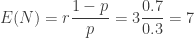
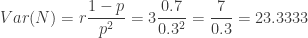
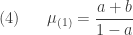
The goal of the above items is to inform on the zero-truncated distribution based on information from the (a,b,0) distribution. They can also be derived based on definitions using the probability function (7). The following shows the factorial means of the zero-truncated distribution.
(12)……..
……..
![\displaystyle \mu_{(1)}=E[N_T]=\frac{a+b}{(1-a) (1-P_0)}](https://s0.wp.com/latex.php?latex=%5Cdisplaystyle+%5Cmu_%7B%281%29%7D%3DE%5BN_T%5D%3D%5Cfrac%7Ba%2Bb%7D%7B%281-a%29+%281-P_0%29%7D&bg=ffffff&fg=333333&s=0&c=20201002)
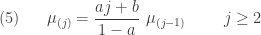
(13)……..
![\displaystyle \begin{aligned} \mu_{(j)}&=E \{ N_T \ [N_T-1] \ [N_T-2] \cdots [N_T-(j-1)] \}\\&\text{ } \\&=\frac{(a j+b) \ \mu_{(j-1)}}{1-a} \end{aligned}](https://s0.wp.com/latex.php?latex=%5Cdisplaystyle+%5Cbegin%7Baligned%7D+%5Cmu_%7B%28j%29%7D%26%3DE+%5C%7B+N_T+%5C+%5BN_T-1%5D+%5C+%5BN_T-2%5D+%5Ccdots+%5BN_T-%28j-1%29%5D+%5C%7D%5C%5C%26%5Ctext%7B+%7D+%5C%5C%26%3D%5Cfrac%7B%28a+j%2Bb%29+%5C+%5Cmu_%7B%28j-1%29%7D%7D%7B1-a%7D++%5Cend%7Baligned%7D&bg=ffffff&fg=333333&s=0&c=20201002)
The first factorial mean is identical to the mean of 
![E[N_T^k]](https://s0.wp.com/latex.php?latex=E%5BN_T%5Ek%5D&bg=ffffff&fg=333333&s=0&c=20201002)
(14)……..
![\displaystyle Var[N_T]=\frac{(a+b) \ [1-(a+b+1) \ P_0]}{[(1-a) \ (1-P_0) ]^2}](https://s0.wp.com/latex.php?latex=%5Cdisplaystyle+Var%5BN_T%5D%3D%5Cfrac%7B%28a%2Bb%29+%5C+%5B1-%28a%2Bb%2B1%29+%5C+P_0%5D%7D%7B%5B%281-a%29+%5C+%281-P_0%29+%5D%5E2%7D&bg=ffffff&fg=333333&s=0&c=20201002)
Example 1
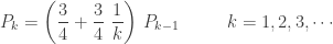
It is helpful to go through an example. First, we set up an (a,b,0) distribution – an negative binomial distribution with parameters 


……….

……….
……….
![\displaystyle E[N]=6](https://s0.wp.com/latex.php?latex=%5Cdisplaystyle+E%5BN%5D%3D6&bg=ffffff&fg=333333&s=0&c=20201002)
……….
![\displaystyle Var[N]=24](https://s0.wp.com/latex.php?latex=%5Cdisplaystyle+Var%5BN%5D%3D24&bg=ffffff&fg=333333&s=0&c=20201002)
……….
![\displaystyle P(z)=[1-3 \ (z-1)]^{-2}](https://s0.wp.com/latex.php?latex=%5Cdisplaystyle+P%28z%29%3D%5B1-3+%5C+%28z-1%29%5D%5E%7B-2%7D&bg=ffffff&fg=333333&s=0&c=20201002)
The following table shows the first 5 probabilities for the zero-truncated negative binomial distribution.
 |
(a,b,0)  |
Zero-Truncated  |
|---|---|---|
| 0 |  |
|
| 1 |  |
 |
| 2 |  |
 |
| 3 | |
|
| 4 |  |
 |
| 5 |  |
 |
The probabilities
……….
![\displaystyle E[N_T]=\frac{16}{15} \ 6=\frac{32}{5}=6.4](https://s0.wp.com/latex.php?latex=%5Cdisplaystyle+E%5BN_T%5D%3D%5Cfrac%7B16%7D%7B15%7D+%5C+6%3D%5Cfrac%7B32%7D%7B5%7D%3D6.4&bg=ffffff&fg=333333&s=0&c=20201002)
……….
![\displaystyle Var[N_T]=\frac{576}{25}=23.04](https://s0.wp.com/latex.php?latex=%5Cdisplaystyle+Var%5BN_T%5D%3D%5Cfrac%7B576%7D%7B25%7D%3D23.04&bg=ffffff&fg=333333&s=0&c=20201002)
……….
![\displaystyle P^T(z)=\frac{16}{15} \biggl( [1-3 \ (z-1)]^{-2}-\frac{1}{16} \biggr)](https://s0.wp.com/latex.php?latex=%5Cdisplaystyle+P%5ET%28z%29%3D%5Cfrac%7B16%7D%7B15%7D+%5Cbiggl%28+%5B1-3+%5C+%28z-1%29%5D%5E%7B-2%7D-%5Cfrac%7B1%7D%7B16%7D+%5Cbiggr%29&bg=ffffff&fg=333333&s=0&c=20201002)
Zero-Modified Distributions
The goal of this section is to derive a zero-modified distribution from a zero-truncated distribution, either derived from an (a,b,0) distribution as discussed in the preceding section, or a truncated distribution not originated from (a,b,0) class.
We now take a zero-truncated distribution as a given and derive the probabilities 
(15)……..
The probability 

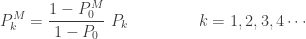
(16)……..

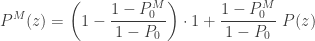
Of course, if the zero-truncated distribution is based on a distribution from the (a,b,0) class, we can express the zero-modified probabilities as, after plugging (7) into (16):
(17)……..
Further distributional quantities can now be derived:
(18)……..

(19)……..
![\displaystyle E[N_M]=(1-P_0^M) \ E[N_T]](https://s0.wp.com/latex.php?latex=%5Cdisplaystyle+E%5BN_M%5D%3D%281-P_0%5EM%29+%5C+E%5BN_T%5D&bg=ffffff&fg=333333&s=0&c=20201002)
(20)……..
![\displaystyle Var[N_M]=(1-P_0^M) \ Var[N_T]+P_0^M \ (1-P_0^M) \ E[N_T]^2](https://s0.wp.com/latex.php?latex=%5Cdisplaystyle+Var%5BN_M%5D%3D%281-P_0%5EM%29+%5C+Var%5BN_T%5D%2BP_0%5EM+%5C+%281-P_0%5EM%29+%5C+E%5BN_T%5D%5E2&bg=ffffff&fg=333333&s=0&c=20201002)
The result (18) is the pgf of the zero-modified distribution based on the pgf of the given zero-truncated distribution. In words, (19) says that the mean of the modified distribution is 

If the given zero-truncated distribution is actually obtained from a member of the (a,b,0) class, then the above three results can be expressed in terms of (a,b,0) information, after plugging the corresponding information for
(21)……..
(22)……..
![\displaystyle E[N_M]=\frac{1-P_0^M}{1-P_0} \ E[N]](https://s0.wp.com/latex.php?latex=%5Cdisplaystyle+E%5BN_M%5D%3D%5Cfrac%7B1-P_0%5EM%7D%7B1-P_0%7D+%5C+E%5BN%5D&bg=ffffff&fg=333333&s=0&c=20201002)
(23)……..
![\displaystyle Var[N_M]=\frac{1-P_0^M}{1-P_0} \ Var[N]+ \biggl(1-\frac{1-P_0^M}{1-P_0} \biggr) \ \frac{1-P_0^M}{1-P_0} \ E[N]^2](https://s0.wp.com/latex.php?latex=%5Cdisplaystyle+Var%5BN_M%5D%3D%5Cfrac%7B1-P_0%5EM%7D%7B1-P_0%7D+%5C+Var%5BN%5D%2B+%5Cbiggl%281-%5Cfrac%7B1-P_0%5EM%7D%7B1-P_0%7D+%5Cbiggr%29+%5C+%5Cfrac%7B1-P_0%5EM%7D%7B1-P_0%7D+%5C+E%5BN%5D%5E2&bg=ffffff&fg=333333&s=0&c=20201002)
Example 2
Consider the zero-truncated negative binomial distribution considered in Example 1. We now generate information on the corresponding zero-modified negative binomial distribution with the assumed value of 
| |
(a,b,0) |
Zero-Truncated |
Zero-Modified  |
|---|---|---|---|
| 0 | |
0.2 | |
| 1 | |
|
 |
| 2 | |
|
 |
| 3 | |
|
|
| 4 | |
|
 |
| 5 | |
|
 |
The zero-modified probabilities 
……….
![\displaystyle E[N_M]=0.8 \ E[N_T]=0.8 (6.4)=5.12](https://s0.wp.com/latex.php?latex=%5Cdisplaystyle+E%5BN_M%5D%3D0.8+%5C+E%5BN_T%5D%3D0.8+%286.4%29%3D5.12&bg=ffffff&fg=333333&s=0&c=20201002)
……….
![\displaystyle Var[N_M]=24.9856](https://s0.wp.com/latex.php?latex=%5Cdisplaystyle+Var%5BN_M%5D%3D24.9856&bg=ffffff&fg=333333&s=0&c=20201002)
……….
![\displaystyle P^M(z)=0.2+0.8 \biggl[ \frac{16}{15} \biggl( [1-3 \ (z-1)]^{-2}-\frac{1}{16} \biggr) \biggr]](https://s0.wp.com/latex.php?latex=%5Cdisplaystyle+P%5EM%28z%29%3D0.2%2B0.8+%5Cbiggl%5B+%5Cfrac%7B16%7D%7B15%7D+%5Cbiggl%28+%5B1-3+%5C+%28z-1%29%5D%5E%7B-2%7D-%5Cfrac%7B1%7D%7B16%7D+%5Cbiggr%29+%5Cbiggr%5D&bg=ffffff&fg=333333&s=0&c=20201002)
Additional Zero-Truncated Distributions
As indicated earlier, the (a,b,1) class contains distributions other than the ones derived from the three (a,b,0) distributions. These distributions also have the zero-truncated versions as well as the zero-modified versions. We discuss the truncated versions. They are: the extended truncated negative binomial (ETNB) distribution, the logarithmic distribution and the Sibuya distribution. The extended truncated negative binomial (ETNB) distribution is resulted from relaxing the r parameter of the negative binomial distribution. The logarithmic distribution and Sibuya distribution are derived from the ETNB distribution. The modified versions of these three distributions can then be obtained by going through the process outlined in the preceding section.
ETNB
Recall that the (a,b,0) negative binomial distribution has two parameters 

……….

……….

The extended negative binomial distribution is resulted from extending the 

(24)……..

What do we do with the ETNB parameters indicated in (24)? Using these ![P_0=[1/(1+\theta)]^r](https://s0.wp.com/latex.php?latex=P_0%3D%5B1%2F%281%2B%5Ctheta%29%5D%5Er&bg=ffffff&fg=333333&s=0&c=20201002)
Using the idea in the preceding paragraph, we can also come up with direct formula for the ETNB probabilities
……….

……….

……….

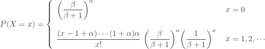
Based on the pattern of the above three probabilities, the ENTB probability 
(25)……..

All other distributional quantities such as pgf and means and higher moments can be derived based on the ETNB pf
(26)……..
![\displaystyle E[N_T]=\frac{1}{1-P_0} \ E[N]=\frac{1}{1-P_0} \ r \ \theta=\frac{r \ \theta}{1-(1+\theta)^{-r}}](https://s0.wp.com/latex.php?latex=%5Cdisplaystyle+E%5BN_T%5D%3D%5Cfrac%7B1%7D%7B1-P_0%7D+%5C+E%5BN%5D%3D%5Cfrac%7B1%7D%7B1-P_0%7D+%5C+r+%5C+%5Ctheta%3D%5Cfrac%7Br+%5C+%5Ctheta%7D%7B1-%281%2B%5Ctheta%29%5E%7B-r%7D%7D&bg=ffffff&fg=333333&s=0&c=20201002)
(27)……..
![\displaystyle \begin{aligned} Var[N_T]&=\frac{1}{1-P_0} \ Var[N]+\biggl(1-\frac{1}{1-P_0} \biggr) \ \frac{1}{1-P_0} \ E[N]^2 \\&=r \ \theta \ \frac{(1+\theta)-(1+\theta+ r \ \theta) \ (1+\theta)^{- r}}{[1-(1+\theta)^{-r}]^2} \end{aligned}](https://s0.wp.com/latex.php?latex=%5Cdisplaystyle+%5Cbegin%7Baligned%7D+Var%5BN_T%5D%26%3D%5Cfrac%7B1%7D%7B1-P_0%7D+%5C+Var%5BN%5D%2B%5Cbiggl%281-%5Cfrac%7B1%7D%7B1-P_0%7D+%5Cbiggr%29+%5C+%5Cfrac%7B1%7D%7B1-P_0%7D+%5C+E%5BN%5D%5E2+%5C%5C%26%3Dr+%5C+%5Ctheta+%5C+%5Cfrac%7B%281%2B%5Ctheta%29-%281%2B%5Ctheta%2B+r+%5C+%5Ctheta%29+%5C+%281%2B%5Ctheta%29%5E%7B-+r%7D%7D%7B%5B1-%281%2B%5Ctheta%29%5E%7B-r%7D%5D%5E2%7D++%5Cend%7Baligned%7D&bg=ffffff&fg=333333&s=0&c=20201002)
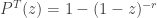
(28)……..
![\displaystyle \begin{aligned} P^T(z)&=\frac{1}{1-P_0} \ (P(z)-P_0) \\&=\frac{1}{1-(1+\theta)^{-r}} \ \biggl[ \biggl(1-\theta (z-1) \biggr)^{-r} -(1+\theta)^{-r}\biggr] \end{aligned}](https://s0.wp.com/latex.php?latex=%5Cdisplaystyle+%5Cbegin%7Baligned%7D+P%5ET%28z%29%26%3D%5Cfrac%7B1%7D%7B1-P_0%7D+%5C+%28P%28z%29-P_0%29+%5C%5C%26%3D%5Cfrac%7B1%7D%7B1-%281%2B%5Ctheta%29%5E%7B-r%7D%7D+%5C+%5Cbiggl%5B+%5Cbiggl%281-%5Ctheta+%28z-1%29+%5Cbiggr%29%5E%7B-r%7D+-%281%2B%5Ctheta%29%5E%7B-r%7D%5Cbiggr%5D++%5Cend%7Baligned%7D&bg=ffffff&fg=333333&s=0&c=20201002)
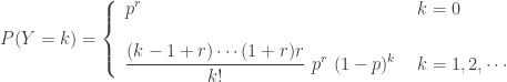
Logarithmic Distribution
This is a truncated distribution that is derived from ETNB by letting 
(29)……..

(30)……..
The parameter 

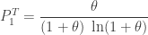
(31)……..
![\displaystyle E[N_T]=\frac{\theta}{\ln(1+\theta) }](https://s0.wp.com/latex.php?latex=%5Cdisplaystyle+E%5BN_T%5D%3D%5Cfrac%7B%5Ctheta%7D%7B%5Cln%281%2B%5Ctheta%29+%7D&bg=ffffff&fg=333333&s=0&c=20201002)
(32)……..
![\displaystyle Var[N_T]=\frac{\theta \biggl[1+\theta-\theta / \ln(1+\theta) \biggr]}{\ln(1+\theta)}](https://s0.wp.com/latex.php?latex=%5Cdisplaystyle+Var%5BN_T%5D%3D%5Cfrac%7B%5Ctheta+%5Cbiggl%5B1%2B%5Ctheta-%5Ctheta+%2F+%5Cln%281%2B%5Ctheta%29++%5Cbiggr%5D%7D%7B%5Cln%281%2B%5Ctheta%29%7D&bg=ffffff&fg=333333&s=0&c=20201002)
Sibuya Distribution
This is a truncated distribution that is derived from ETNB by letting 
(33)……..

(34)……..
All of the three items are obtained by letting 
……….
![\displaystyle P_1^T=\frac{r \theta}{(1+\theta)^{r+1}-(1+\theta)}=\frac{r \theta}{(1+\theta) \ [(1+\theta)^r-1]}=r \ \frac{\theta}{1+\theta} \ \frac{1}{(1+\theta)^r-1}](https://s0.wp.com/latex.php?latex=%5Cdisplaystyle+P_1%5ET%3D%5Cfrac%7Br+%5Ctheta%7D%7B%281%2B%5Ctheta%29%5E%7Br%2B1%7D-%281%2B%5Ctheta%29%7D%3D%5Cfrac%7Br+%5Ctheta%7D%7B%281%2B%5Ctheta%29+%5C+%5B%281%2B%5Ctheta%29%5Er-1%5D%7D%3Dr+%5C+%5Cfrac%7B%5Ctheta%7D%7B1%2B%5Ctheta%7D+%5C+%5Cfrac%7B1%7D%7B%281%2B%5Ctheta%29%5Er-1%7D&bg=ffffff&fg=333333&s=0&c=20201002)
As 


(35)……..
Once these three zero-truncated distributions are obtained, we can derive the zero-modified versions of these distributions in the process described earlier.
Example 3
We demonstrate how ETNB is calculated. Let 
……….

The 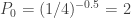
| |
Artificial |
Zero-Truncated  |
|---|---|---|
| 0 |  |
|
| 1 |  |
 |
| 2 |  |
 |
| 3 |  |
 |
| 4 |  |
 |
| 5 |  |
 |
The column labeled artificial 
Using (26) and (27), the ETNB mean and variance are ![E[N_T]=3/2](https://s0.wp.com/latex.php?latex=E%5BN_T%5D%3D3%2F2&bg=ffffff&fg=333333&s=0&c=20201002)
![Var[N_T]=3/2](https://s0.wp.com/latex.php?latex=Var%5BN_T%5D%3D3%2F2&bg=ffffff&fg=333333&s=0&c=20201002)

| |
Artificial |
Zero-Truncated |
Zero-Modified  |
|---|---|---|---|
| 0 | |
0.1 | |
| 1 | |
|
 |
| 2 | |
|
 |
| 3 | |
|
 |
| 4 | |
|
 |
| 5 | |
|
 |
With the assumed value of 
![E[N_M]=1.35](https://s0.wp.com/latex.php?latex=E%5BN_M%5D%3D1.35&bg=ffffff&fg=333333&s=0&c=20201002)
![Var[N_M]=1.5525](https://s0.wp.com/latex.php?latex=Var%5BN_M%5D%3D1.5525&bg=ffffff&fg=333333&s=0&c=20201002)
Practice Problems
The discussion in this post has a great deal of technical details. A concise summary of the (a,b,0) class and (a,b,1) class is found here.
Practice problems on (a,b,0) class
Practice problems on (a,b,1) class
Dan Ma actuarial topics
Dan Ma actuarial
Dan Ma math
Daniel Ma actuarial
Daniel Ma mathematics
Daniel Ma actuarial topics

 , let
, let  . The counting random variable
 starting at 1. The relation (1) does not account for

![\displaystyle W=\biggl[ 1+(a+b)+\biggl(a+\frac{b}{2} \biggr)(a+b)+\cdots+ \biggl \{ \biggl(a+\frac{b}{k} \biggr) \cdots \biggl(a+\frac{b}{2} \biggr)(a+b) \biggr \} +\cdots \biggr]](https://s0.wp.com/latex.php?latex=%5Cdisplaystyle+W%3D%5Cbiggl%5B+1%2B%28a%2Bb%29%2B%5Cbiggl%28a%2B%5Cfrac%7Bb%7D%7B2%7D+%5Cbiggr%29%28a%2Bb%29%2B%5Ccdots%2B+%5Cbiggl+%5C%7B+%5Cbiggl%28a%2B%5Cfrac%7Bb%7D%7Bk%7D+%5Cbiggr%29+%5Ccdots+%5Cbiggl%28a%2B%5Cfrac%7Bb%7D%7B2%7D+%5Cbiggr%29%28a%2Bb%29+%5Cbiggr+%5C%7D+%2B%5Ccdots+%5Cbiggr%5D&bg=ffffff&fg=333333&s=0&c=20201002)
 and
and  where
where  is a fixed positive constant. Using (1), we see that


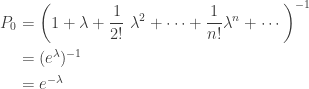
 are from a Poisson distribution. Thus, when the parameter
 and
and 


 and
and  . The two rows for negative binomial reflect two different parametrizations. Of course, the geometric distribution is simply a negative binomial distribution when the parameter
  . Essentially Table 1 consists of three different distributions.
 , the resulting probabilities
  ,
,  , i.e. the distribution is a point mass at 0. So we would like to restrict the attention on the case where
  .
.


 and
and  . Since
  and
and  . With this information, the (a,b,0) distribution in question is completely determined. The following are the several distributional quantities.
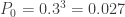


 and
and  . Since
 and
and  . The (a,b,0) distribution in question is then completely determined.
 , its
, its ![(3) \ \ \ \ \ \mu_{(n)}=E[X (X-1) (X-2) \cdots (X-(n-1))]](https://s0.wp.com/latex.php?latex=%283%29+%5C+%5C+%5C+%5C+%5C+%5Cmu_%7B%28n%29%7D%3DE%5BX+%28X-1%29+%28X-2%29+%5Ccdots+%28X-%28n-1%29%29%5D&bg=ffffff&fg=333333&s=0&c=20201002)
![\mu_{(1)}=E[X]](https://s0.wp.com/latex.php?latex=%5Cmu_%7B%281%29%7D%3DE%5BX%5D&bg=ffffff&fg=333333&s=0&c=20201002)
![\mu_{(2)}=E[X (X-1)]](https://s0.wp.com/latex.php?latex=%5Cmu_%7B%282%29%7D%3DE%5BX+%28X-1%29%5D&bg=ffffff&fg=333333&s=0&c=20201002)
![\mu_{(3)}=E[X (X-1) (X-2)]](https://s0.wp.com/latex.php?latex=%5Cmu_%7B%283%29%7D%3DE%5BX+%28X-1%29+%28X-2%29%5D&bg=ffffff&fg=333333&s=0&c=20201002)
![\displaystyle \mu_{(1)}=E[N]=\frac{a+b}{1-a}](https://s0.wp.com/latex.php?latex=%5Cdisplaystyle+%5Cmu_%7B%281%29%7D%3DE%5BN%5D%3D%5Cfrac%7Ba%2Bb%7D%7B1-a%7D&bg=ffffff&fg=333333&s=0&c=20201002)
![\displaystyle \mu_{(2)}=\frac{2 a +b}{1-a} \ \frac{a+b}{1-a}=\frac{(2a+b) (a+b)}{(1-a)^2}=E[N (N-1)]=E[N^2]-E[N]](https://s0.wp.com/latex.php?latex=%5Cdisplaystyle+%5Cmu_%7B%282%29%7D%3D%5Cfrac%7B2+a+%2Bb%7D%7B1-a%7D+%5C+%5Cfrac%7Ba%2Bb%7D%7B1-a%7D%3D%5Cfrac%7B%282a%2Bb%29+%28a%2Bb%29%7D%7B%281-a%29%5E2%7D%3DE%5BN+%28N-1%29%5D%3DE%5BN%5E2%5D-E%5BN%5D&bg=ffffff&fg=333333&s=0&c=20201002)
![\displaystyle E[N^2]=\frac{(2a+b) (a+b)}{(1-a)^2}+\frac{a+b}{1-a}=\frac{(a+b) (a+b+1)}{(1-a)^2}](https://s0.wp.com/latex.php?latex=%5Cdisplaystyle+E%5BN%5E2%5D%3D%5Cfrac%7B%282a%2Bb%29+%28a%2Bb%29%7D%7B%281-a%29%5E2%7D%2B%5Cfrac%7Ba%2Bb%7D%7B1-a%7D%3D%5Cfrac%7B%28a%2Bb%29+%28a%2Bb%2B1%29%7D%7B%281-a%29%5E2%7D&bg=ffffff&fg=333333&s=0&c=20201002)
![\displaystyle Var(N)=E[N^2]-E[N]^2=\frac{a+b}{(1-a)^2}](https://s0.wp.com/latex.php?latex=%5Cdisplaystyle+Var%28N%29%3DE%5BN%5E2%5D-E%5BN%5D%5E2%3D%5Cfrac%7Ba%2Bb%7D%7B%281-a%29%5E2%7D&bg=ffffff&fg=333333&s=0&c=20201002)

 is the observed frequency for the category
  multiplied by
  be a random variable with positive probabilities only on the non-negative integers, i.e.
  is positive only for
  , i.e. the observed value of the random variable
 . The generating function
  is defined wherever the infinite sum converges. At minimum,
  . Some
  , e.g. when
  .
.![\displaystyle E[Y (Y-1) (Y-2) \cdots (Y-(n-1)]=P_Y^{(n)}(1)](https://s0.wp.com/latex.php?latex=%5Cdisplaystyle+E%5BY+%28Y-1%29+%28Y-2%29+%5Ccdots+%28Y-%28n-1%29%5D%3DP_Y%5E%7B%28n%29%7D%281%29&bg=ffffff&fg=333333&s=0&c=20201002)
 . Since
 ![E[Y (Y-1)]=P_Y^{(2)}(1)](https://s0.wp.com/latex.php?latex=E%5BY+%28Y-1%29%5D%3DP_Y%5E%7B%282%29%7D%281%29&bg=ffffff&fg=333333&s=0&c=20201002) , the second moment is
, the second moment is  . In general, the
  can be expressed in terms of
  for all
  .
. .
.
 . Another useful property about generating function is that the probability distribution of a random variable is uniquely determined by its generating function. This fundamental property is useful in determining the distribution of an independent sum. The generating function of an independent sum of random variables is simply the product of the individual generating functions. If the product is the generating function of a certain distribution, then the independent sum must be of the same distribution.
 .
.
![E[X (X-1)]=P_X^{(2)}(1)=\lambda^2](https://s0.wp.com/latex.php?latex=E%5BX+%28X-1%29%5D%3DP_X%5E%7B%282%29%7D%281%29%3D%5Clambda%5E2&bg=ffffff&fg=333333&s=0&c=20201002)
![E[X^2]=P_X^{(1)}(1)+P_X^{(2)}(1)=\lambda+\lambda^2](https://s0.wp.com/latex.php?latex=E%5BX%5E2%5D%3DP_X%5E%7B%281%29%7D%281%29%2BP_X%5E%7B%282%29%7D%281%29%3D%5Clambda%2B%5Clambda%5E2&bg=ffffff&fg=333333&s=0&c=20201002)

 are independent Poisson random variables with means
  , respectively. Then the probability generating function of the sum
  is simply the product of the individual probability generating functions.
 . The probability generating function of the sum
  distinct types such that the probability of a claim being of type
  is
is  ,
,  and such that
  . If we are interested in studying the number
  of claims in a year that are of type
  , then
  are independent Poisson random variables with means
  , respectively. For a mathematical discussion of this Poisson splitting phenomenon, see
  is the number of Success in the
 raised to
 is defined for all real values
![E[X (X-1)]=n (n-1) p^2](https://s0.wp.com/latex.php?latex=E%5BX+%28X-1%29%5D%3Dn+%28n-1%29+p%5E2&bg=ffffff&fg=333333&s=0&c=20201002)
 .
.  , where each
  has a binomial distribution with parameters
  and
and  and
and 
 is computed by its usual definition. The above probability probability function can be relaxed so that
 does not have to be an integer. If
  would lead to the same calculation. The reformulation is a generalization of the usual binomial coefficient definition.

 originate from the parameters of the gamma distribution in the Poisson-gamma mixture. The mean and variance are:

 to denote the mapping. For example, if
  is a number that is intended to quantify the risk exposure. We first look at some examples.
![\rho(X)=E[X]](https://s0.wp.com/latex.php?latex=%5Crho%28X%29%3DE%5BX%5D&bg=ffffff&fg=333333&s=0&c=20201002) ………………………………………………….(Equivalence Principle)
………………………………………………….(Equivalence Principle)
![\rho(X)=(1+k) \ E[X]](https://s0.wp.com/latex.php?latex=%5Crho%28X%29%3D%281%2Bk%29+%5C+E%5BX%5D&bg=ffffff&fg=333333&s=0&c=20201002) ……………………………………….(Expected Value Principle)
……………………………………….(Expected Value Principle)![\rho(X)=E[X]+ k \ Var(X)](https://s0.wp.com/latex.php?latex=%5Crho%28X%29%3DE%5BX%5D%2B+k+%5C+Var%28X%29&bg=ffffff&fg=333333&s=0&c=20201002) …………………………………(Variance Principle)
…………………………………(Variance Principle) …………………………………..(Standard Deviation Principle)
 . The fixed constant
![\mu=E[X]](https://s0.wp.com/latex.php?latex=%5Cmu%3DE%5BX%5D&bg=ffffff&fg=333333&s=0&c=20201002) and
and  is the variance of
  ,
,  . This means that
  is a threshold that indicates the level of adverse outcome such that the probability of exceeding this threshold is 5%. With
  ,
,  . The higher threshold
  is the level of adverse outcome so that there is a 1% chance of exceeding it.
 th percentile. The corresponding
  is the
  , is the expected loss on the condition that loss exceeds the 100pth percentile of
 . Tail-value-at-risk is a risk measure that is in many ways superior than VaR. The risk measure VaR is a merely a cutoff point and does not describe the tail behavior beyond the VaR threshold. TVaR reflects the shape of the tail beyond VaR threshold. See
  ……………………………………….(Subadditivity)
 with probability 1, then
  ………………..(Monotonicity)
 ,
,  ………………………(Positive Homogeneity)
 ……………….(Translation Invariance)
 be no greater than the risk measures for
 .
.


 .
.

 where
where  represents the random losses and
 , i.e. the risk
  . There is no benefit of risk reduction in combing risks that are positively correlated.
 , we can find random variables
  . To this end, we define random variables
  and
and  and
and  . Let
. Let  . Then it is straightforward to verify that


 , the constant
  as
as 
 always and
  . Thus monotonicity fails for the variance principle.

 . This is derived by the following:
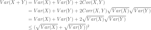
 refers to the correlation coefficient, which is always
  . The following shows the subadditivity.
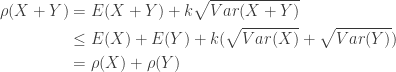
 , we show that for each
  and
and  where
where  is the positive number defined by
  . Let
. Let 

 , the constant
  as
as  (however small), we can always find an integer
  . Thus monotonicity fails for the standard deviation principle.
 .
. , VaR at the security level
  and
and  , with weights
  and
and  , respectively. Let
  be the
 ![\displaystyle \begin{aligned} \text{TVaR}_p(X)&=\pi_p+\frac{1}{1-p} \biggl[w \times P(X_1>\pi_p) \times e_{X_1}(\pi_p)\\& \ \ +(1-w) \times P(X_2>\pi_p) \times e_{X_2}(\pi_p)\biggr] \ \ \ \ \ \ \ \ \ \ \ \ \ \ \ (a) \end{aligned}](https://s0.wp.com/latex.php?latex=%5Cdisplaystyle+%5Cbegin%7Baligned%7D+%5Ctext%7BTVaR%7D_p%28X%29%26%3D%5Cpi_p%2B%5Cfrac%7B1%7D%7B1-p%7D+%5Cbiggl%5Bw+%5Ctimes+P%28X_1%3E%5Cpi_p%29+%5Ctimes+e_%7BX_1%7D%28%5Cpi_p%29%5C%5C%26++%5C+%5C++%2B%281-w%29+%5Ctimes+P%28X_2%3E%5Cpi_p%29++%5Ctimes+e_%7BX_2%7D%28%5Cpi_p%29%5Cbiggr%5D++%5C+%5C+%5C+%5C+%5C+%5C+%5C+%5C+%5C+%5C+%5C+%5C+%5C+%5C+%5C+%28a%29+%5Cend%7Baligned%7D&bg=ffffff&fg=333333&s=0&c=20201002)
 . In other words, TVaR is VaR plus the mean excess loss function evaluated at
  and
and  . This formula is useful if the
 , we solve the following equation.
 . Then solve for
  . The following is the 99th percentile of the loss
![\displaystyle \begin{aligned} \text{TVaR}_p(X)&=\pi_p+\frac{1}{1-0.99} \biggl[0.75 \times e^{-\pi_p/5} \times 5 +0.25 \times e^{-\pi_p/10} \times 10 \biggr] \\&=42.7283 \end{aligned}](https://s0.wp.com/latex.php?latex=%5Cdisplaystyle+%5Cbegin%7Baligned%7D+%5Ctext%7BTVaR%7D_p%28X%29%26%3D%5Cpi_p%2B%5Cfrac%7B1%7D%7B1-0.99%7D+%5Cbiggl%5B0.75+%5Ctimes+e%5E%7B-%5Cpi_p%2F5%7D+%5Ctimes+5+%2B0.25+%5Ctimes+e%5E%7B-%5Cpi_p%2F10%7D+%5Ctimes+10+%5Cbiggr%5D+%5C%5C%26%3D42.7283++%5Cend%7Baligned%7D&bg=ffffff&fg=333333&s=0&c=20201002)
 and the density function for
  . The density function of
  . We derive from the basic definition of TVaR. Let
 ![\displaystyle \begin{aligned} \text{TVaR}_p(X)&=\frac{\int_{\pi_p}^\infty x f(x) \ dx}{1-p}\\&=\pi_p+\frac{\int_{\pi_p}^\infty (x-\pi_p) f(x) \ dx}{1-p} \\&=\pi_p+\frac{\int_{\pi_p}^\infty (x-\pi_p) (w f_1(x)+(1-w) f_2(x)) \ dx}{1-p} \\&=\pi_p+\frac{1}{1-p} \biggl[w \int_{\pi_p}^\infty (x-\pi_p) f_1(x) \ dx +(1-w) \int_{\pi_p}^\infty (x-\pi_p) f_2(x) \ dx\biggr] \\&=\pi_p+\frac{1}{1-p} \biggl[w \ P(X_1>\pi_p) \ \frac{\int_{\pi_p}^\infty (x-\pi_p) f_1(x) \ dx}{P(X_1>\pi_p)}\\& \ \ +(1-w) \ P(X_2>\pi_p) \ \frac{\int_{\pi_p}^\infty (x-\pi_p) f_2(x) \ dx}{P(X_2>\pi_p)} \biggr] \\&=\pi_p+\frac{1}{1-p} \biggl[w \ P(X_1>\pi_p) \ e_{X_1}(\pi_p) +(1-w) \ P(X_2>\pi_p) \ e_{X_2}(\pi_p) \biggr] \end{aligned}](https://s0.wp.com/latex.php?latex=%5Cdisplaystyle+%5Cbegin%7Baligned%7D+%5Ctext%7BTVaR%7D_p%28X%29%26%3D%5Cfrac%7B%5Cint_%7B%5Cpi_p%7D%5E%5Cinfty+x+f%28x%29+%5C+dx%7D%7B1-p%7D%5C%5C%26%3D%5Cpi_p%2B%5Cfrac%7B%5Cint_%7B%5Cpi_p%7D%5E%5Cinfty+%28x-%5Cpi_p%29+f%28x%29+%5C+dx%7D%7B1-p%7D+%5C%5C%26%3D%5Cpi_p%2B%5Cfrac%7B%5Cint_%7B%5Cpi_p%7D%5E%5Cinfty+%28x-%5Cpi_p%29+%28w+f_1%28x%29%2B%281-w%29+f_2%28x%29%29+%5C+dx%7D%7B1-p%7D+%5C%5C%26%3D%5Cpi_p%2B%5Cfrac%7B1%7D%7B1-p%7D+%5Cbiggl%5Bw+%5Cint_%7B%5Cpi_p%7D%5E%5Cinfty+%28x-%5Cpi_p%29+f_1%28x%29+%5C+dx+%2B%281-w%29+%5Cint_%7B%5Cpi_p%7D%5E%5Cinfty+%28x-%5Cpi_p%29+f_2%28x%29+%5C+dx%5Cbiggr%5D+%5C%5C%26%3D%5Cpi_p%2B%5Cfrac%7B1%7D%7B1-p%7D+%5Cbiggl%5Bw+%5C+++P%28X_1%3E%5Cpi_p%29+%5C+%5Cfrac%7B%5Cint_%7B%5Cpi_p%7D%5E%5Cinfty+%28x-%5Cpi_p%29+f_1%28x%29+%5C+dx%7D%7BP%28X_1%3E%5Cpi_p%29%7D%5C%5C%26+%5C+%5C++%2B%281-w%29+%5C+P%28X_2%3E%5Cpi_p%29+%5C+%5Cfrac%7B%5Cint_%7B%5Cpi_p%7D%5E%5Cinfty+%28x-%5Cpi_p%29+f_2%28x%29+%5C+dx%7D%7BP%28X_2%3E%5Cpi_p%29%7D+%5Cbiggr%5D+%5C%5C%26%3D%5Cpi_p%2B%5Cfrac%7B1%7D%7B1-p%7D+%5Cbiggl%5Bw+%5C+++P%28X_1%3E%5Cpi_p%29+%5C+e_%7BX_1%7D%28%5Cpi_p%29+%2B%281-w%29+%5C+P%28X_2%3E%5Cpi_p%29+%5C+e_%7BX_2%7D%28%5Cpi_p%29+%5Cbiggr%5D+%5Cend%7Baligned%7D&bg=ffffff&fg=333333&s=0&c=20201002)
 . In some ways, VaR is an attractive risk measure. Mathematically speaking, VaR has a clear and simple definition. For certain probability models, VaR can be evaluated in closed form. For those models that have no closed form for percentiles, VaR can be evaluated using software. However, VaR has limitations (this point will be briefly discussed below).
 and variance
  where
where  is the
  for some fixed constant
  and
and  .
.

 where
where  is the cumulative distribution function (CDF) of
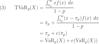
 is the mean excess loss function evaluated at
  , the following is a useful formulation for TVaR.
![\displaystyle \begin{aligned} (4) \ \ \ \ \ \text{TVaR}_p(X)&=\text{VaR}_p(X)+e(\text{VaR}_p(X)) \\&=\text{VaR}_p(X)+\frac{E[X]-E[X \wedge \text{VaR}_p(X)]}{1-p} \end{aligned}](https://s0.wp.com/latex.php?latex=%5Cdisplaystyle+%5Cbegin%7Baligned%7D+%284%29+%5C+%5C+%5C+%5C+%5C+%5Ctext%7BTVaR%7D_p%28X%29%26%3D%5Ctext%7BVaR%7D_p%28X%29%2Be%28%5Ctext%7BVaR%7D_p%28X%29%29+%5C%5C%26%3D%5Ctext%7BVaR%7D_p%28X%29%2B%5Cfrac%7BE%5BX%5D-E%5BX+%5Cwedge+%5Ctext%7BVaR%7D_p%28X%29%5D%7D%7B1-p%7D+%5Cend%7Baligned%7D&bg=ffffff&fg=333333&s=0&c=20201002)


![\displaystyle \frac{\theta}{\alpha-1} \biggl[1+ \frac{\alpha}{\theta} \ \text{VaR}_p(X) \biggr]](https://s0.wp.com/latex.php?latex=%5Cdisplaystyle+%5Cfrac%7B%5Ctheta%7D%7B%5Calpha-1%7D+%5Cbiggl%5B1%2B+%5Cfrac%7B%5Calpha%7D%7B%5Ctheta%7D+%5C+%5Ctext%7BVaR%7D_p%28X%29+%5Cbiggr%5D&bg=ffffff&fg=333333&s=0&c=20201002)


![\displaystyle e^{\mu+0.5 \ \sigma^2} \biggl[\frac{\Phi(\sigma-z_p)}{1-p} \biggr]](https://s0.wp.com/latex.php?latex=%5Cdisplaystyle+e%5E%7B%5Cmu%2B0.5+%5C+%5Csigma%5E2%7D+%5Cbiggl%5B%5Cfrac%7B%5CPhi%28%5Csigma-z_p%29%7D%7B1-p%7D+%5Cbiggr%5D&bg=ffffff&fg=333333&s=0&c=20201002)
 and a scale parameter
  (standard deviation). The lognormal distribution are parametrized by
  and
and  are the probability density function and the cumulative distribution function of the standard normal distribution, respectively. Thus
 is evaluated by using a table or software and not by evaluating the integral.
 in the integrand is always positive. The area in between the curve
  . When this expression is normalized, i.e. divided by
 is defined over all positive
  . The integral of
 , the results are the exponential distributions. When
  and
and  where
where  is defined by the integral
  where
where  is the density function of the distribution in question. If the distribution puts significantly more probabilities in the larger values in the right tail, this integral may not exist (may not converge) for some
  , the Pareto variance does not exist. This shows that for a heavy tailed distribution, the variance may not be a good measure of risk.
 of a random variable
 (Pareto Type I) and
  (Pareto Type II Lomax). Both hazard rates are decreasing function.
  , the Weibull hazard rate is decreasing and when
  , the hazard rate is increasing. When
  , Weibull is the exponential distribution, which has a constant hazard rate.
 , which is called the cumulative hazard rate function. As indicated above,
  . If
. If  has a lower rate of increase and consequently
  . If the random variable
  is an ordinary deductible that is part of an insurance coverage. Then
  is the expected payment made by the insurer in the event that the loss exceeds the deductible.
 , which is increasing. The mean excess loss for Pareto Type II Lomax is
  , which is also decreasing. They are both increasing functions of the deductible
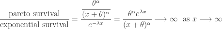
  captures the probability of the tail of a distribution. If a distribution whose survival function decays slowly to zero (equivalently the cdf goes slowly to one), it is another indication that the distribution is heavy tailed. This point is touched on when discussing hazard rate function.
 and
and  . The following table is a comparison of the two survival functions.
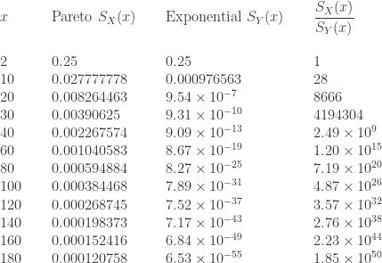
 .
. is an exponential distribution with
  being a rate parameter. When
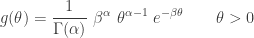
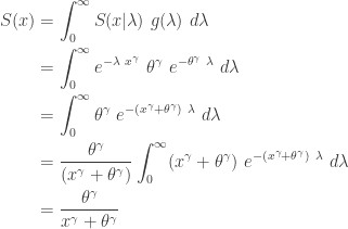
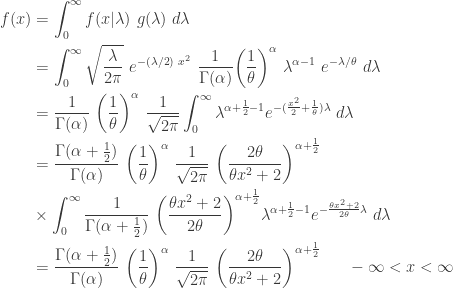
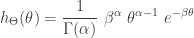
![\displaystyle g(\theta)=\frac{1}{\Gamma(\alpha)} \ \biggl[\frac{\beta}{\theta}\biggr]^\alpha \ \frac{1}{\theta} \ e^{-\frac{\beta}{ \theta}} \ \ \ \ \ \theta>0](https://s0.wp.com/latex.php?latex=%5Cdisplaystyle+g%28%5Ctheta%29%3D%5Cfrac%7B1%7D%7B%5CGamma%28%5Calpha%29%7D+%5C+%5Cbiggl%5B%5Cfrac%7B%5Cbeta%7D%7B%5Ctheta%7D%5Cbiggr%5D%5E%5Calpha+%5C+%5Cfrac%7B1%7D%7B%5Ctheta%7D+%5C+e%5E%7B-%5Cfrac%7B%5Cbeta%7D%7B+%5Ctheta%7D%7D+%5C+%5C+%5C+%5C+%5C+%5Ctheta%3E0&bg=ffffff&fg=333333&s=0&c=20201002)
![\displaystyle \begin{aligned} S(x)&=\int_0^\infty S(x \lvert \theta) \ g(\theta) \ d \theta \\&=\int_0^\infty e^{- x/\theta} \ \frac{1}{\Gamma(\alpha)} \ \biggl[\frac{\beta}{\theta}\biggr]^\alpha \ \frac{1}{\theta} \ e^{-\beta / \theta} \ d \theta \\&=\int_0^\infty \frac{1}{\Gamma(\alpha)} \ \biggl[\frac{\beta}{\theta}\biggr]^\alpha \ \frac{1}{\theta} \ e^{-(x+\beta) / \theta} \ d \theta \\&=\frac{\beta^\alpha}{(x+\beta)^\alpha} \ \int_0^\infty \frac{1}{\Gamma(\alpha)} \ \biggl[\frac{x+\beta}{\theta}\biggr]^\alpha \ \frac{1}{\theta} \ e^{-(x+\beta) / \theta} \ d \theta \\&=\biggl(\frac{\beta}{x+\beta} \biggr)^\alpha \end{aligned}](https://s0.wp.com/latex.php?latex=%5Cdisplaystyle+%5Cbegin%7Baligned%7D+S%28x%29%26%3D%5Cint_0%5E%5Cinfty+S%28x+%5Clvert+%5Ctheta%29+%5C+g%28%5Ctheta%29+%5C+d+%5Ctheta+%5C%5C%26%3D%5Cint_0%5E%5Cinfty+e%5E%7B-+x%2F%5Ctheta%7D+%5C+%5Cfrac%7B1%7D%7B%5CGamma%28%5Calpha%29%7D+%5C+%5Cbiggl%5B%5Cfrac%7B%5Cbeta%7D%7B%5Ctheta%7D%5Cbiggr%5D%5E%5Calpha+%5C+%5Cfrac%7B1%7D%7B%5Ctheta%7D+%5C+e%5E%7B-%5Cbeta+%2F+%5Ctheta%7D+%5C+d+%5Ctheta+%5C%5C%26%3D%5Cint_0%5E%5Cinfty+%5Cfrac%7B1%7D%7B%5CGamma%28%5Calpha%29%7D+%5C+%5Cbiggl%5B%5Cfrac%7B%5Cbeta%7D%7B%5Ctheta%7D%5Cbiggr%5D%5E%5Calpha+%5C+%5Cfrac%7B1%7D%7B%5Ctheta%7D+%5C+e%5E%7B-%28x%2B%5Cbeta%29+%2F+%5Ctheta%7D+%5C+d+%5Ctheta+%5C%5C%26%3D%5Cfrac%7B%5Cbeta%5E%5Calpha%7D%7B%28x%2B%5Cbeta%29%5E%5Calpha%7D+%5C+%5Cint_0%5E%5Cinfty+%5Cfrac%7B1%7D%7B%5CGamma%28%5Calpha%29%7D+%5C+%5Cbiggl%5B%5Cfrac%7Bx%2B%5Cbeta%7D%7B%5Ctheta%7D%5Cbiggr%5D%5E%5Calpha+%5C+%5Cfrac%7B1%7D%7B%5Ctheta%7D+%5C+e%5E%7B-%28x%2B%5Cbeta%29+%2F+%5Ctheta%7D+%5C+d+%5Ctheta+%5C%5C%26%3D%5Cbiggl%28%5Cfrac%7B%5Cbeta%7D%7Bx%2B%5Cbeta%7D+%5Cbiggr%29%5E%5Calpha+%5Cend%7Baligned%7D&bg=ffffff&fg=333333&s=0&c=20201002)
 , the following is the density function of


 has a simple expression
  when
when  .
.  , the conditional distribution for
  and
and  degrees of freedom is the generalized Pareto distribution with parameters
  ,
,  and
and  . As a result, the following is the density function.
 has a Weibull distribution with shape parameter
  (a known constant) and a parameter
  such that the CDF of
 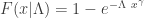 . Further suppose that the random parameter
  . Then the unconditional distribution for
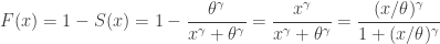
![\displaystyle f(x)=\frac{d}{dx} \biggl( \frac{x^\gamma}{x^\gamma+\theta^\gamma} \biggr)=\frac{\gamma \ (x/\theta)^\gamma}{x [1+(x/\theta)^\gamma]^2}](https://s0.wp.com/latex.php?latex=%5Cdisplaystyle+f%28x%29%3D%5Cfrac%7Bd%7D%7Bdx%7D+%5Cbiggl%28+%5Cfrac%7Bx%5E%5Cgamma%7D%7Bx%5E%5Cgamma%2B%5Ctheta%5E%5Cgamma%7D+%5Cbiggr%29%3D%5Cfrac%7B%5Cgamma+%5C+%28x%2F%5Ctheta%29%5E%5Cgamma%7D%7Bx+%5B1%2B%28x%2F%5Ctheta%29%5E%5Cgamma%5D%5E2%7D&bg=ffffff&fg=333333&s=0&c=20201002)
 . Then
  .
.![\displaystyle \begin{aligned} P[Y \le y]&=P[\frac{1}{X} \le y] =P[X \ge y^{-1}] =\frac{\theta^\gamma}{y^{-\gamma}+\theta^\gamma} \\&=\frac{\theta^\gamma \ y^\gamma}{1+\theta^\gamma \ y^\gamma} \\&=\frac{y^\gamma}{(\theta^{-1})^\gamma+y^\gamma} \end{aligned}](https://s0.wp.com/latex.php?latex=%5Cdisplaystyle+%5Cbegin%7Baligned%7D+P%5BY+%5Cle+y%5D%26%3DP%5B%5Cfrac%7B1%7D%7BX%7D+%5Cle+y%5D+%3DP%5BX+%5Cge+y%5E%7B-1%7D%5D+%3D%5Cfrac%7B%5Ctheta%5E%5Cgamma%7D%7By%5E%7B-%5Cgamma%7D%2B%5Ctheta%5E%5Cgamma%7D+%5C%5C%26%3D%5Cfrac%7B%5Ctheta%5E%5Cgamma+%5C+y%5E%5Cgamma%7D%7B1%2B%5Ctheta%5E%5Cgamma+%5C+y%5E%5Cgamma%7D+%5C%5C%26%3D%5Cfrac%7By%5E%5Cgamma%7D%7B%28%5Ctheta%5E%7B-1%7D%29%5E%5Cgamma%2By%5E%5Cgamma%7D+%5Cend%7Baligned%7D&bg=ffffff&fg=333333&s=0&c=20201002)
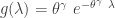
 . According to formula (4) in
 ![\displaystyle E[ (X \lvert \Lambda)^k]=\Gamma \biggl(1+\frac{k}{\gamma} \biggr) \Lambda^{-k/\gamma}](https://s0.wp.com/latex.php?latex=%5Cdisplaystyle+E%5B+%28X+%5Clvert+%5CLambda%29%5Ek%5D%3D%5CGamma+%5Cbiggl%281%2B%5Cfrac%7Bk%7D%7B%5Cgamma%7D+%5Cbiggr%29+%5CLambda%5E%7B-k%2F%5Cgamma%7D&bg=ffffff&fg=333333&s=0&c=20201002)
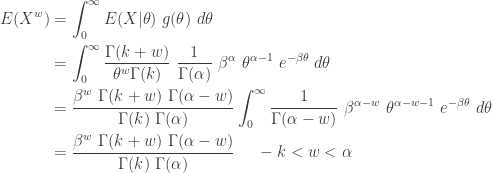
![\displaystyle \begin{aligned} E[X^k]&=\int_0^\infty E[ (X \lvert \Lambda)^k] \ g(\lambda) \ d \lambda \\&=\int_0^\infty \Gamma \biggl(1+\frac{k}{\gamma} \biggr) \lambda^{-k/\gamma} \ \theta^\gamma \ e^{-\theta^\gamma \ \lambda} \ d \lambda\\&=\Gamma \biggl(1+\frac{k}{\gamma} \biggr) \ \theta^\gamma \int_0^\infty \lambda^{-k/\gamma} \ e^{-\theta^\gamma \ \lambda} \ d \lambda \\&=\theta^k \ \Gamma \biggl(1+\frac{k}{\gamma} \biggr) \int_0^\infty t^{-k/\gamma} \ e^{-t} \ dt \ \ \text{ where } t=\theta^\gamma \lambda \\&=\theta^k \ \Gamma \biggl(1+\frac{k}{\gamma} \biggr) \int_0^\infty t^{[(\gamma-k)/\gamma]-1} \ e^{-t} \ dt \\&=\theta^k \ \Gamma \biggl(1+\frac{k}{\gamma} \biggr) \ \Gamma \biggl(1-\frac{k}{\gamma} \biggr) \ \ \ \ -\gamma<k<\gamma \end{aligned}](https://s0.wp.com/latex.php?latex=%5Cdisplaystyle+%5Cbegin%7Baligned%7D+E%5BX%5Ek%5D%26%3D%5Cint_0%5E%5Cinfty+E%5B+%28X+%5Clvert+%5CLambda%29%5Ek%5D+%5C+g%28%5Clambda%29+%5C+d+%5Clambda+%5C%5C%26%3D%5Cint_0%5E%5Cinfty+%5CGamma+%5Cbiggl%281%2B%5Cfrac%7Bk%7D%7B%5Cgamma%7D+%5Cbiggr%29+%5Clambda%5E%7B-k%2F%5Cgamma%7D+%5C+%5Ctheta%5E%5Cgamma+%5C+e%5E%7B-%5Ctheta%5E%5Cgamma+%5C+%5Clambda%7D+%5C+d+%5Clambda%5C%5C%26%3D%5CGamma+%5Cbiggl%281%2B%5Cfrac%7Bk%7D%7B%5Cgamma%7D+%5Cbiggr%29+%5C+%5Ctheta%5E%5Cgamma+%5Cint_0%5E%5Cinfty++%5Clambda%5E%7B-k%2F%5Cgamma%7D+%5C+e%5E%7B-%5Ctheta%5E%5Cgamma+%5C+%5Clambda%7D+%5C+d+%5Clambda+%5C%5C%26%3D%5Ctheta%5Ek+%5C+%5CGamma+%5Cbiggl%281%2B%5Cfrac%7Bk%7D%7B%5Cgamma%7D+%5Cbiggr%29++%5Cint_0%5E%5Cinfty++t%5E%7B-k%2F%5Cgamma%7D+%5C+e%5E%7B-t%7D+%5C+dt+%5C+%5C+%5Ctext%7B+where+%7D+t%3D%5Ctheta%5E%5Cgamma+%5Clambda+%5C%5C%26%3D%5Ctheta%5Ek+%5C+%5CGamma+%5Cbiggl%281%2B%5Cfrac%7Bk%7D%7B%5Cgamma%7D+%5Cbiggr%29+%5Cint_0%5E%5Cinfty++t%5E%7B%5B%28%5Cgamma-k%29%2F%5Cgamma%5D-1%7D+%5C+e%5E%7B-t%7D+%5C+dt+++%5C%5C%26%3D%5Ctheta%5Ek+%5C+%5CGamma+%5Cbiggl%281%2B%5Cfrac%7Bk%7D%7B%5Cgamma%7D+%5Cbiggr%29+%5C+%5CGamma+%5Cbiggl%281-%5Cfrac%7Bk%7D%7B%5Cgamma%7D+%5Cbiggr%29+%5C+%5C+%5C+%5C+-%5Cgamma%3Ck%3C%5Cgamma++%5Cend%7Baligned%7D&bg=ffffff&fg=333333&s=0&c=20201002)
 follows from the fact that the arguments of the gamma function must be positive. Thus the
  , then
  has a gamma distribution with shape parameter
 ![P[Y=\alpha]=p (1-p)^{\alpha-1}](https://s0.wp.com/latex.php?latex=P%5BY%3D%5Calpha%5D%3Dp+%281-p%29%5E%7B%5Calpha-1%7D&bg=ffffff&fg=333333&s=0&c=20201002) where
where  . Then the unconditional distribution for
  .
.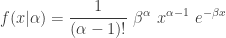
![\displaystyle \begin{aligned} f(x)&=\sum \limits_{\alpha=1}^\infty f(x \lvert \alpha) \ P[Y=\alpha] \\&=\sum \limits_{\alpha=1}^\infty \frac{1}{(\alpha-1)!} \ \beta^\alpha \ x^{\alpha-1} \ e^{-\beta x} \ p (1-p)^{\alpha-1} \\&=\beta p \ e^{-\beta x} \sum \limits_{\alpha=1}^\infty \frac{[\beta(1-p) x]^{\alpha-1}}{(\alpha-1)!} \\&=\beta p \ e^{-\beta x} \sum \limits_{\alpha=0}^\infty \frac{[\beta(1-p) x]^{\alpha}}{(\alpha)!} \\&=\beta p \ e^{-\beta x} \ e^{\beta(1-p) x} \end{aligned}](https://s0.wp.com/latex.php?latex=%5Cdisplaystyle+%5Cbegin%7Baligned%7D+f%28x%29%26%3D%5Csum+%5Climits_%7B%5Calpha%3D1%7D%5E%5Cinfty+f%28x+%5Clvert+%5Calpha%29+%5C+P%5BY%3D%5Calpha%5D+%5C%5C%26%3D%5Csum+%5Climits_%7B%5Calpha%3D1%7D%5E%5Cinfty+%5Cfrac%7B1%7D%7B%28%5Calpha-1%29%21%7D+%5C+%5Cbeta%5E%5Calpha+%5C+x%5E%7B%5Calpha-1%7D+%5C+e%5E%7B-%5Cbeta+x%7D+%5C+p+%281-p%29%5E%7B%5Calpha-1%7D+%5C%5C%26%3D%5Cbeta+p+%5C+e%5E%7B-%5Cbeta+x%7D+%5Csum+%5Climits_%7B%5Calpha%3D1%7D%5E%5Cinfty+%5Cfrac%7B%5B%5Cbeta%281-p%29+x%5D%5E%7B%5Calpha-1%7D%7D%7B%28%5Calpha-1%29%21%7D+%5C%5C%26%3D%5Cbeta+p+%5C+e%5E%7B-%5Cbeta+x%7D+%5Csum+%5Climits_%7B%5Calpha%3D0%7D%5E%5Cinfty+%5Cfrac%7B%5B%5Cbeta%281-p%29+x%5D%5E%7B%5Calpha%7D%7D%7B%28%5Calpha%29%21%7D+%5C%5C%26%3D%5Cbeta+p+%5C+e%5E%7B-%5Cbeta+x%7D+%5C+e%5E%7B%5Cbeta%281-p%29+x%7D+%5Cend%7Baligned%7D&bg=ffffff&fg=333333&s=0&c=20201002)
 . Further suppose that the random parameter
  is a positive integer. Then the unconditional distribution for
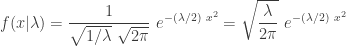

 and
and  . The following derivation converts to the common
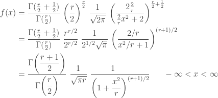
 where
where  (if
(if  (if
(if 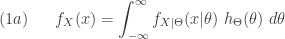
 is a weighted average of a family of pdfs
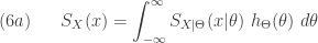
 or cumulative distribution function
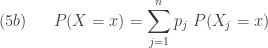
  is a weighted average of a family of probability functions or cumulative distributions indexed by the mixing random variable


 (continuous case)
 (discrete case)
 where the sum of the
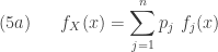
![\displaystyle (7) \ \ \ \ \ Var(X)=E[Var(X \lvert \Theta)]+Var[E(X \lvert \Theta)]](https://s0.wp.com/latex.php?latex=%5Cdisplaystyle+%287%29+%5C+%5C+%5C+%5C+%5C+Var%28X%29%3DE%5BVar%28X+%5Clvert+%5CTheta%29%5D%2BVar%5BE%28X+%5Clvert+%5CTheta%29%5D&bg=ffffff&fg=333333&s=0&c=20201002)
 . The first component
 ![E[Var(X \lvert \Theta)]](https://s0.wp.com/latex.php?latex=E%5BVar%28X+%5Clvert+%5CTheta%29%5D&bg=ffffff&fg=333333&s=0&c=20201002) is called the expected value of conditional variances, which is the weighted average of the conditional variances. The second component
is called the expected value of conditional variances, which is the weighted average of the conditional variances. The second component ![Var[E(X \lvert \Theta)]](https://s0.wp.com/latex.php?latex=Var%5BE%28X+%5Clvert+%5CTheta%29%5D&bg=ffffff&fg=333333&s=0&c=20201002) is called the variance of the conditional means, which represents the additional variance as a result of the uncertainty in the parameter
is called the variance of the conditional means, which represents the additional variance as a result of the uncertainty in the parameter  , the variation will be reflected in
  where
where 
 and
and  are known parameters of the gamma distribution. Then the unconditional pdf of

 . This is one form of a negative binomial distribution. The mean is
  and the variance is
  . The variance of the negative binomial distribution is greater than the mean. In a Poisson distribution, the mean equals the variance. Thus the unconditional claim frequency
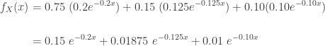

 . The pdf and cdf of the mixture will allow us to derive other distributional quantities such as moments and then using the moments to derive skewness and kurtosis. The moments for exponential distribution has a closed form. Then the moments of the mixture distribution is simply the weighted average of the exponential moments.
![\displaystyle E(X^k)=0.75 \ [5^k \ k!]+0.15 \ [8^k \ k!]+0.10 \ [10^k \ k!]](https://s0.wp.com/latex.php?latex=%5Cdisplaystyle+E%28X%5Ek%29%3D0.75+%5C+%5B5%5Ek+%5C+k%21%5D%2B0.15+%5C+%5B8%5Ek+%5C+k%21%5D%2B0.10+%5C+%5B10%5Ek+%5C+k%21%5D&bg=ffffff&fg=333333&s=0&c=20201002)


 . The three conditional exponential variances are 25, 64 and 100. The weighted average of these would be 38.35. Because of the uncertainty resulting from not knowing which exponential distribution the claim is from, the unconditional variance is larger than 38.35.
![\displaystyle \gamma=E\biggl[\biggl( \frac{X-\mu}{\sigma} \biggr)^3\biggr]=\frac{E(X^3)-3 \mu \sigma^2-\mu^3}{(\sigma^2)^{1.5}}](https://s0.wp.com/latex.php?latex=%5Cdisplaystyle+%5Cgamma%3DE%5Cbiggl%5B%5Cbiggl%28+%5Cfrac%7BX-%5Cmu%7D%7B%5Csigma%7D+%5Cbiggr%29%5E3%5Cbiggr%5D%3D%5Cfrac%7BE%28X%5E3%29-3+%5Cmu+%5Csigma%5E2-%5Cmu%5E3%7D%7B%28%5Csigma%5E2%29%5E%7B1.5%7D%7D&bg=ffffff&fg=333333&s=0&c=20201002)
![\displaystyle \text{Kurt}[X]=E\biggl[\biggl( \frac{X-\mu}{\sigma} \biggr)^4\biggr]=\frac{E(X^4)-4 \mu E(X^3)+6 \mu^2 E(X^2)-3 \mu^4}{\sigma^4}](https://s0.wp.com/latex.php?latex=%5Cdisplaystyle+%5Ctext%7BKurt%7D%5BX%5D%3DE%5Cbiggl%5B%5Cbiggl%28+%5Cfrac%7BX-%5Cmu%7D%7B%5Csigma%7D+%5Cbiggr%29%5E4%5Cbiggr%5D%3D%5Cfrac%7BE%28X%5E4%29-4+%5Cmu+E%28X%5E3%29%2B6+%5Cmu%5E2+E%28X%5E2%29-3+%5Cmu%5E4%7D%7B%5Csigma%5E4%7D&bg=ffffff&fg=333333&s=0&c=20201002)
 and
and  . The expressions on the right hand side are in terms of the raw moments
  . Plugging in the raw moments produces the skewness
  and kurtosis
 ![\text{Kurt}[X]=14.0097](https://s0.wp.com/latex.php?latex=%5Ctext%7BKurt%7D%5BX%5D%3D14.0097&bg=ffffff&fg=333333&s=0&c=20201002) . The excess kurtosis is then 11.0097 (subtracting 3 from the kurtosis).
. The excess kurtosis is then 11.0097 (subtracting 3 from the kurtosis).  , where
  , conditional on the parameter
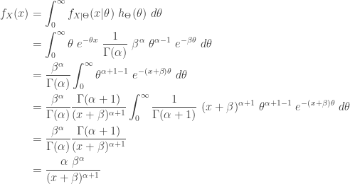
 where
where ![\displaystyle f_{X \lvert \Theta}(x \lvert \theta)=\frac{1}{\sqrt{2 \pi v}} \ \text{exp}\biggl[-\frac{1}{2v}(x-\theta)^2 \biggr] \ \ \ -\infty<x<\infty](https://s0.wp.com/latex.php?latex=%5Cdisplaystyle+f_%7BX+%5Clvert+%5CTheta%7D%28x+%5Clvert+%5Ctheta%29%3D%5Cfrac%7B1%7D%7B%5Csqrt%7B2+%5Cpi+v%7D%7D+%5C+%5Ctext%7Bexp%7D%5Cbiggl%5B-%5Cfrac%7B1%7D%7B2v%7D%28x-%5Ctheta%29%5E2+%5Cbiggr%5D+%5C+%5C+%5C+-%5Cinfty%3Cx%3C%5Cinfty&bg=ffffff&fg=333333&s=0&c=20201002)
![\displaystyle f_{\Theta}(\theta)=\frac{1}{\sqrt{2 \pi a}} \ \text{exp}\biggl[-\frac{1}{2a}(\theta-\mu)^2 \biggr] \ \ \ -\infty<x<\infty](https://s0.wp.com/latex.php?latex=%5Cdisplaystyle+f_%7B%5CTheta%7D%28%5Ctheta%29%3D%5Cfrac%7B1%7D%7B%5Csqrt%7B2+%5Cpi+a%7D%7D+%5C+%5Ctext%7Bexp%7D%5Cbiggl%5B-%5Cfrac%7B1%7D%7B2a%7D%28%5Ctheta-%5Cmu%29%5E2+%5Cbiggr%5D+%5C+%5C+%5C+-%5Cinfty%3Cx%3C%5Cinfty&bg=ffffff&fg=333333&s=0&c=20201002)
![\displaystyle \begin{aligned} f_X(x)&=\int_{-\infty}^\infty \frac{1}{\sqrt{2 \pi v}} \ \text{exp}\biggl[-\frac{1}{2v}(x-\theta)^2 \biggr] \ \frac{1}{\sqrt{2 \pi a}} \ \text{exp}\biggl[-\frac{1}{2a}(\theta-\mu)^2 \biggr] \ d \theta \\&=\frac{1}{2 \pi \sqrt{va}} \int_{-\infty}^\infty \text{exp}\biggl[-\frac{1}{2v}(x-\theta)^2 -\frac{1}{2a}(\theta-\mu)^2\biggr] \ d \theta \end{aligned}](https://s0.wp.com/latex.php?latex=%5Cdisplaystyle+%5Cbegin%7Baligned%7D+f_X%28x%29%26%3D%5Cint_%7B-%5Cinfty%7D%5E%5Cinfty+%5Cfrac%7B1%7D%7B%5Csqrt%7B2+%5Cpi+v%7D%7D+%5C+%5Ctext%7Bexp%7D%5Cbiggl%5B-%5Cfrac%7B1%7D%7B2v%7D%28x-%5Ctheta%29%5E2+%5Cbiggr%5D+%5C+%5Cfrac%7B1%7D%7B%5Csqrt%7B2+%5Cpi+a%7D%7D+%5C+%5Ctext%7Bexp%7D%5Cbiggl%5B-%5Cfrac%7B1%7D%7B2a%7D%28%5Ctheta-%5Cmu%29%5E2+%5Cbiggr%5D+%5C+d+%5Ctheta+%5C%5C%26%3D%5Cfrac%7B1%7D%7B2+%5Cpi+%5Csqrt%7Bva%7D%7D+%5Cint_%7B-%5Cinfty%7D%5E%5Cinfty+%5Ctext%7Bexp%7D%5Cbiggl%5B-%5Cfrac%7B1%7D%7B2v%7D%28x-%5Ctheta%29%5E2+-%5Cfrac%7B1%7D%7B2a%7D%28%5Ctheta-%5Cmu%29%5E2%5Cbiggr%5D+%5C+d+%5Ctheta++%5Cend%7Baligned%7D&bg=ffffff&fg=333333&s=0&c=20201002)
![\displaystyle \frac{(x-\theta)^2}{v}+\frac{(\theta-\mu)^2}{a}=\frac{a+v}{va} \biggl[\theta-\frac{ax+v \mu}{a+v}\biggr]^2 +\frac{(x-\mu)^2}{a+v}](https://s0.wp.com/latex.php?latex=%5Cdisplaystyle+%5Cfrac%7B%28x-%5Ctheta%29%5E2%7D%7Bv%7D%2B%5Cfrac%7B%28%5Ctheta-%5Cmu%29%5E2%7D%7Ba%7D%3D%5Cfrac%7Ba%2Bv%7D%7Bva%7D+%5Cbiggl%5B%5Ctheta-%5Cfrac%7Bax%2Bv+%5Cmu%7D%7Ba%2Bv%7D%5Cbiggr%5D%5E2+%2B%5Cfrac%7B%28x-%5Cmu%29%5E2%7D%7Ba%2Bv%7D+&bg=ffffff&fg=333333&s=0&c=20201002)
![\displaystyle \begin{aligned} f_X(x)&=\frac{1}{2 \pi \sqrt{va}} \int_{-\infty}^\infty \text{exp}\biggl[-\frac{1}{2} \biggl(\frac{a+v}{va} \biggl[\theta-\frac{ax+v \mu}{a+v}\biggr]^2 +\frac{(x-\mu)^2}{a+v} \biggr) \biggr] \ d \theta \\&\displaystyle =\frac{\text{exp}\biggl[\displaystyle -\frac{(x-\mu)^2}{2(a+v)} \biggr]}{2 \pi \sqrt{va}} \int_{-\infty}^\infty \text{exp}\biggl[\displaystyle -\frac{1}{2} \biggl(\frac{a+v}{va} \biggl[\theta-\frac{ax+v \mu}{a+v}\biggr]^2 \biggr) \biggr] \ d \theta \\&=\frac{\text{exp}\biggl[\displaystyle -\frac{(x-\mu)^2}{2(a+v)} \biggr]}{\sqrt{2 \pi (a+v)} } \int_{-\infty}^\infty \frac{1}{\sqrt{2 \pi}} \sqrt{\frac{a+v}{va}} \ \text{exp}\biggl[-\frac{1}{2} \biggl(\frac{a+v}{va} \biggl[\theta-\frac{ax+v \mu}{a+v}\biggr]^2 \biggr) \biggr] \ d \theta \\&=\frac{\text{exp}\biggl[\displaystyle -\frac{(x-\mu)^2}{2(a+v)} \biggr]}{\sqrt{2 \pi (a+v)} } \end{aligned}](https://s0.wp.com/latex.php?latex=%5Cdisplaystyle+%5Cbegin%7Baligned%7D+f_X%28x%29%26%3D%5Cfrac%7B1%7D%7B2+%5Cpi+%5Csqrt%7Bva%7D%7D+%5Cint_%7B-%5Cinfty%7D%5E%5Cinfty+%5Ctext%7Bexp%7D%5Cbiggl%5B-%5Cfrac%7B1%7D%7B2%7D+%5Cbiggl%28%5Cfrac%7Ba%2Bv%7D%7Bva%7D+%5Cbiggl%5B%5Ctheta-%5Cfrac%7Bax%2Bv+%5Cmu%7D%7Ba%2Bv%7D%5Cbiggr%5D%5E2+%2B%5Cfrac%7B%28x-%5Cmu%29%5E2%7D%7Ba%2Bv%7D++%5Cbiggr%29+%5Cbiggr%5D+%5C+d+%5Ctheta+%5C%5C%26%5Cdisplaystyle+%3D%5Cfrac%7B%5Ctext%7Bexp%7D%5Cbiggl%5B%5Cdisplaystyle+-%5Cfrac%7B%28x-%5Cmu%29%5E2%7D%7B2%28a%2Bv%29%7D+%5Cbiggr%5D%7D%7B2+%5Cpi+%5Csqrt%7Bva%7D%7D++%5Cint_%7B-%5Cinfty%7D%5E%5Cinfty++%5Ctext%7Bexp%7D%5Cbiggl%5B%5Cdisplaystyle+-%5Cfrac%7B1%7D%7B2%7D+%5Cbiggl%28%5Cfrac%7Ba%2Bv%7D%7Bva%7D+%5Cbiggl%5B%5Ctheta-%5Cfrac%7Bax%2Bv+%5Cmu%7D%7Ba%2Bv%7D%5Cbiggr%5D%5E2+%5Cbiggr%29+%5Cbiggr%5D+%5C+d+%5Ctheta+%5C%5C%26%3D%5Cfrac%7B%5Ctext%7Bexp%7D%5Cbiggl%5B%5Cdisplaystyle+-%5Cfrac%7B%28x-%5Cmu%29%5E2%7D%7B2%28a%2Bv%29%7D+%5Cbiggr%5D%7D%7B%5Csqrt%7B2+%5Cpi+%28a%2Bv%29%7D+%7D++%5Cint_%7B-%5Cinfty%7D%5E%5Cinfty+%5Cfrac%7B1%7D%7B%5Csqrt%7B2+%5Cpi%7D%7D+%5Csqrt%7B%5Cfrac%7Ba%2Bv%7D%7Bva%7D%7D+%5C+%5Ctext%7Bexp%7D%5Cbiggl%5B-%5Cfrac%7B1%7D%7B2%7D+%5Cbiggl%28%5Cfrac%7Ba%2Bv%7D%7Bva%7D+%5Cbiggl%5B%5Ctheta-%5Cfrac%7Bax%2Bv+%5Cmu%7D%7Ba%2Bv%7D%5Cbiggr%5D%5E2+%5Cbiggr%29+%5Cbiggr%5D+%5C+d+%5Ctheta+%5C%5C%26%3D%5Cfrac%7B%5Ctext%7Bexp%7D%5Cbiggl%5B%5Cdisplaystyle+-%5Cfrac%7B%28x-%5Cmu%29%5E2%7D%7B2%28a%2Bv%29%7D+%5Cbiggr%5D%7D%7B%5Csqrt%7B2+%5Cpi+%28a%2Bv%29%7D+%7D++%5Cend%7Baligned%7D&bg=ffffff&fg=333333&s=0&c=20201002)
 and variance
  . Hence the integral is 1. The last expression is the unconditional pdf of
 ![\displaystyle f_X(x)=\frac{1}{\sqrt{2 \pi (a+v)}} \ \text{exp}\biggl[-\frac{(x-\mu)^2}{2(a+v)} \biggr] \ \ \ \ -\infty<x<\infty](https://s0.wp.com/latex.php?latex=%5Cdisplaystyle+f_X%28x%29%3D%5Cfrac%7B1%7D%7B%5Csqrt%7B2+%5Cpi+%28a%2Bv%29%7D%7D+%5C+%5Ctext%7Bexp%7D%5Cbiggl%5B-%5Cfrac%7B%28x-%5Cmu%29%5E2%7D%7B2%28a%2Bv%29%7D+%5Cbiggr%5D+%5C+%5C+%5C+%5C+-%5Cinfty%3Cx%3C%5Cinfty&bg=ffffff&fg=333333&s=0&c=20201002)
 . Thus the mixing normal distribution with mean
  be a positive constant. The random variables
  ,
,  and
and  are called transformed, inverse and inverse transformed, respectively.
 and
and  be the probability density function (PDF), the cumulative distribution function (CDF) and the survival function of the random variable


 is integer
 , which is the
  , the resulting distribution is a transformed Pareto distribution and is also called a Burr distribution, which then is a distribution with three parameters –
  , the resulting distribution is an inverse transformed Pareto distribution and it is also called an inverse Burr distribution. When raising
  , the resulting distribution is a paralogistic distribution. By equating
  and then raise it to the power
  .
.

![\displaystyle f_Y(y)=\frac{\alpha \ \tau \ (y/\theta)^\tau}{y \ [(y/\theta)^\tau+1 ]^{\alpha+1}}](https://s0.wp.com/latex.php?latex=%5Cdisplaystyle+f_Y%28y%29%3D%5Cfrac%7B%5Calpha+%5C+%5Ctau+%5C+%28y%2F%5Ctheta%29%5E%5Ctau%7D%7By+%5C+%5B%28y%2F%5Ctheta%29%5E%5Ctau%2B1+%5D%5E%7B%5Calpha%2B1%7D%7D&bg=ffffff&fg=333333&s=0&c=20201002)

 , else 0

 , which is derived using the Pareto moments. The Burr CDF has a closed form that is relatively easy to compute. Thus percentiles are very accessible. The moments rely on the gamma function and are usually calculated by software.
 . Both ways derive the same CDF. As in the preceding case, we take the latter approach.
 .
.
![\displaystyle f_Y(y)=\frac{\alpha \ \tau \ (y/\theta)^{\tau \alpha}}{y \ [1+(y/\theta)^\tau]^{\alpha+1}}](https://s0.wp.com/latex.php?latex=%5Cdisplaystyle+f_Y%28y%29%3D%5Cfrac%7B%5Calpha+%5C+%5Ctau+%5C+%28y%2F%5Ctheta%29%5E%7B%5Ctau+%5Calpha%7D%7D%7By+%5C+%5B1%2B%28y%2F%5Ctheta%29%5E%5Ctau%5D%5E%7B%5Calpha%2B1%7D%7D&bg=ffffff&fg=333333&s=0&c=20201002)


![\displaystyle \theta \ \biggl[\frac{1}{ 2^{1/\alpha}-1} \biggr]^{1/\tau}](https://s0.wp.com/latex.php?latex=%5Cdisplaystyle+%5Ctheta+%5C+%5Cbiggl%5B%5Cfrac%7B1%7D%7B+2%5E%7B1%2F%5Calpha%7D-1%7D+%5Cbiggr%5D%5E%7B1%2F%5Ctau%7D&bg=ffffff&fg=333333&s=0&c=20201002)
 , else 0


![\displaystyle f_Y(y)=\frac{\alpha^2 \ \ (y/\theta)^\alpha}{y \ [(y/\theta)^\alpha+1 ]^{\alpha+1}}](https://s0.wp.com/latex.php?latex=%5Cdisplaystyle+f_Y%28y%29%3D%5Cfrac%7B%5Calpha%5E2+%5C+%5C+%28y%2F%5Ctheta%29%5E%5Calpha%7D%7By+%5C+%5B%28y%2F%5Ctheta%29%5E%5Calpha%2B1+%5D%5E%7B%5Calpha%2B1%7D%7D&bg=ffffff&fg=333333&s=0&c=20201002)

 , else 0


![\displaystyle f_Y(y)=\frac{\alpha^2 \ (y/\theta)^{\alpha^2}}{y \ [1+(y/\theta)^\alpha]^{\alpha+1}}](https://s0.wp.com/latex.php?latex=%5Cdisplaystyle+f_Y%28y%29%3D%5Cfrac%7B%5Calpha%5E2+%5C+%28y%2F%5Ctheta%29%5E%7B%5Calpha%5E2%7D%7D%7By+%5C+%5B1%2B%28y%2F%5Ctheta%29%5E%5Calpha%5D%5E%7B%5Calpha%2B1%7D%7D&bg=ffffff&fg=333333&s=0&c=20201002)


![\displaystyle \theta \ \biggl[\frac{1}{ 2^{1/\alpha}-1} \biggr]^{1/\alpha}](https://s0.wp.com/latex.php?latex=%5Cdisplaystyle+%5Ctheta+%5C+%5Cbiggl%5B%5Cfrac%7B1%7D%7B+2%5E%7B1%2F%5Calpha%7D-1%7D+%5Cbiggr%5D%5E%7B1%2F%5Calpha%7D&bg=ffffff&fg=333333&s=0&c=20201002)

 , else 0

![\displaystyle f_Y(y)=\frac{\alpha \ \theta \ y^{\alpha-1}}{[\theta+y ]^{\alpha+1}}](https://s0.wp.com/latex.php?latex=%5Cdisplaystyle+f_Y%28y%29%3D%5Cfrac%7B%5Calpha+%5C+%5Ctheta+%5C+y%5E%7B%5Calpha-1%7D%7D%7B%5B%5Ctheta%2By+%5D%5E%7B%5Calpha%2B1%7D%7D&bg=ffffff&fg=333333&s=0&c=20201002)


 is nonexistent.