
This post continues with the discussion on the exponential distribution. The previous posts on the exponential distribution are an introduction, a post on the relation with the Poisson process and a post on more properties. This post discusses the hyperexponential distribution and the hypoexponential distribution.
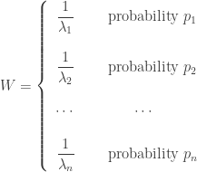
Suppose 


What if the exponential 


To contrast, a hyperexponential distribution is also a “sum” of independent exponential random variables 


The Erlang distribution, the hypoexponential distribution and the hyperexponential distribution are special cases of phase-type distributions that are useful in queuing theory. These distributions are models for interarrival times or service times in queuing systems. They are obtained by breaking down the total time into a number of phases, each having an exponential distribution, where the parameters of the exponential distributions may be identical or may be different. Furthermore, the phases may be in series or in parallel (or both). The phases are in series means that the phases are run sequentially, one at a time. The Erlang distribution is one example of a phase-type distribution where the
The Erlang distribution is a special case of the gamma distribution. For basic properties of the Erlang distribution, see the previous posts on the gamma distribution, starting with this post. The remainder of the post focuses on some basic properties of the hyper and hypo exponential distributions.
_______________________________________________________________________________________________
The Hyperexponential Distribution
The hyperexponential distribution is the mixture of a set of independent exponential distributions. To generate a hyperexponential distribution, let 


Basic facts about mixture distributions can give a great deal of information on the hyperexponential distribution. For example, many distributional quantities of a mixture distribution are obtained by taking weighted averages of the corresponding quantities of the individual components. Specifically, the density function, the cumulative distribution function (CDF), the survival function, along with the mean, the higher moments can all be obtained by taking weighted averages. However, the the variance of a mixture is not the weighted average of the individual variances. The following shows the probability density function 


The above three distributional quantities are the weighted averages of the corresponding quantities of the individual exponential distributions. The hyperexponential distribution is sometimes called a finite mixture since there are a finite number of components in the weighted average. The raw moments of the hyperexponential distribution are also weighted averages of the corresponding exponential raw moments. The following shows the mean and the higher moments ![E[X^k]](https://s0.wp.com/latex.php?latex=E%5BX%5Ek%5D&bg=ffffff&fg=333333&s=0&c=20201002)

![\displaystyle E[X]=p_1 \cdot \biggl(\frac{1}{\lambda_1} \biggr)+p_2 \cdot \biggl(\frac{1}{\lambda_2} \biggr)+\cdots+p_n \cdot \biggl(\frac{1}{\lambda_n} \biggr) \ \ \ \ \ \ \ \ \ \ \ \ \ \ \ \ \ \ \ \ \ \ \ \ \ \ \ \ \ \ (4)](https://s0.wp.com/latex.php?latex=%5Cdisplaystyle+E%5BX%5D%3Dp_1+%5Ccdot+%5Cbiggl%28%5Cfrac%7B1%7D%7B%5Clambda_1%7D+%5Cbiggr%29%2Bp_2+%5Ccdot+%5Cbiggl%28%5Cfrac%7B1%7D%7B%5Clambda_2%7D+%5Cbiggr%29%2B%5Ccdots%2Bp_n+%5Ccdot+%5Cbiggl%28%5Cfrac%7B1%7D%7B%5Clambda_n%7D+%5Cbiggr%29+%5C+%5C+%5C+%5C+%5C+%5C+%5C+%5C+%5C+%5C+%5C+%5C+%5C+%5C+%5C+%5C+%5C+%5C+%5C+%5C+%5C+%5C+%5C+%5C+%5C+%5C+%5C+%5C+%5C+%5C+%284%29&bg=ffffff&fg=333333&s=0&c=20201002)
![\displaystyle E[X^k]=p_1 \cdot \biggl(\frac{k!}{\lambda_1^k} \biggr)+p_2 \cdot \biggl(\frac{k!}{\lambda_2^k} \biggr)+\cdots+p_n \cdot \biggl(\frac{k!}{\lambda_n^k} \biggr) \ \ \ \ \ \ \ \ \ \ \ \ \ \ \ \ \ \ \ \ \ \ \ \ \ \ \ \ \ (5)](https://s0.wp.com/latex.php?latex=%5Cdisplaystyle+E%5BX%5Ek%5D%3Dp_1+%5Ccdot+%5Cbiggl%28%5Cfrac%7Bk%21%7D%7B%5Clambda_1%5Ek%7D+%5Cbiggr%29%2Bp_2+%5Ccdot+%5Cbiggl%28%5Cfrac%7Bk%21%7D%7B%5Clambda_2%5Ek%7D+%5Cbiggr%29%2B%5Ccdots%2Bp_n+%5Ccdot+%5Cbiggl%28%5Cfrac%7Bk%21%7D%7B%5Clambda_n%5Ek%7D+%5Cbiggr%29+%5C+%5C+%5C+%5C+%5C+%5C+%5C+%5C+%5C+%5C+%5C+%5C+%5C+%5C+%5C+%5C+%5C+%5C+%5C+%5C+%5C+%5C+%5C+%5C+%5C+%5C+%5C+%5C+%5C+%285%29&bg=ffffff&fg=333333&s=0&c=20201002)
Interestingly, the hyperexponential variance is not the weighted average of the individual variances.
![\displaystyle Var[X] \ne \sum \limits_{i=1}^n \ p_i \biggl(\frac{1}{\lambda_i^2} \biggr) \ \ \ \ \ \ \ \ \ \ \ \ \ \ \ \ \ \ \ \ \ \ \ \ \ \ \ \ \ \ \ \ \ \ \ \ \ \ \ \ \ \ \ \ \ \ \ \ \ \ \ \ \ \ \ \ \ \ \ \ \ \ \ \ \ (6)](https://s0.wp.com/latex.php?latex=%5Cdisplaystyle+Var%5BX%5D+%5Cne+%5Csum+%5Climits_%7Bi%3D1%7D%5En+%5C+p_i+%5Cbiggl%28%5Cfrac%7B1%7D%7B%5Clambda_i%5E2%7D+%5Cbiggr%29+%5C+%5C+%5C+%5C+%5C+%5C+%5C+%5C+%5C+%5C+%5C+%5C+%5C+%5C+%5C+%5C+%5C+%5C+%5C+%5C+%5C+%5C+%5C+%5C+%5C+%5C+%5C+%5C+%5C+%5C+%5C+%5C+%5C+%5C+%5C+%5C+%5C+%5C+%5C+%5C+%5C+%5C+%5C+%5C+%5C+%5C+%5C+%5C+%5C+%5C+%5C+%5C+%5C+%5C+%5C+%5C+%5C+%5C+%5C+%5C+%5C+%5C+%5C+%5C+%5C+%286%29&bg=ffffff&fg=333333&s=0&c=20201002)
The following gives the correct variance of the hyperexponential distribution.
![\displaystyle Var[X]=E[X^2]-E[X]^2=\sum \limits_{i=1}^n \ p_i \biggl(\frac{2}{\lambda_i^2} \biggr)-\biggl(\sum \limits_{i=1}^n \ p_i \frac{1}{\lambda_i} \biggr)^2 \ \ \ \ \ \ \ \ \ \ \ \ \ \ \ \ \ \ \ \ (7)](https://s0.wp.com/latex.php?latex=%5Cdisplaystyle+Var%5BX%5D%3DE%5BX%5E2%5D-E%5BX%5D%5E2%3D%5Csum+%5Climits_%7Bi%3D1%7D%5En+%5C+p_i+%5Cbiggl%28%5Cfrac%7B2%7D%7B%5Clambda_i%5E2%7D+%5Cbiggr%29-%5Cbiggl%28%5Csum+%5Climits_%7Bi%3D1%7D%5En+%5C+p_i+%5Cfrac%7B1%7D%7B%5Clambda_i%7D+%5Cbiggr%29%5E2+%5C+%5C+%5C+%5C+%5C+%5C+%5C+%5C+%5C+%5C+%5C+%5C+%5C+%5C+%5C+%5C+%5C+%5C+%5C+%5C+%287%29&bg=ffffff&fg=333333&s=0&c=20201002)
It is instructive to rearrange the above variance as follows:
![\displaystyle \begin{aligned} Var[X]&=\sum \limits_{i=1}^n \ p_i \biggl(\frac{2}{\lambda_i^2} \biggr)-\biggl(\sum \limits_{i=1}^n \ p_i \frac{1}{\lambda_i} \biggr)^2 \\&=\sum \limits_{i=1}^n \ p_i \biggl(\frac{1}{\lambda_i^2} \biggr)+\biggl[ \sum \limits_{i=1}^n \ p_i \biggl(\frac{1}{\lambda_i^2} \biggr)-\biggl(\sum \limits_{i=1}^n \ p_i \frac{1}{\lambda_i} \biggr)^2 \biggr] \ \ \ \ \ \ \ \ \ \ \ \ \ \ \ \ \ \ \ \ (8) \end{aligned}](https://s0.wp.com/latex.php?latex=%5Cdisplaystyle+%5Cbegin%7Baligned%7D+Var%5BX%5D%26%3D%5Csum+%5Climits_%7Bi%3D1%7D%5En+%5C+p_i+%5Cbiggl%28%5Cfrac%7B2%7D%7B%5Clambda_i%5E2%7D+%5Cbiggr%29-%5Cbiggl%28%5Csum+%5Climits_%7Bi%3D1%7D%5En+%5C+p_i+%5Cfrac%7B1%7D%7B%5Clambda_i%7D+%5Cbiggr%29%5E2+%5C%5C%26%3D%5Csum+%5Climits_%7Bi%3D1%7D%5En+%5C+p_i+%5Cbiggl%28%5Cfrac%7B1%7D%7B%5Clambda_i%5E2%7D+%5Cbiggr%29%2B%5Cbiggl%5B+%5Csum+%5Climits_%7Bi%3D1%7D%5En+%5C+p_i+%5Cbiggl%28%5Cfrac%7B1%7D%7B%5Clambda_i%5E2%7D+%5Cbiggr%29-%5Cbiggl%28%5Csum+%5Climits_%7Bi%3D1%7D%5En+%5C+p_i+%5Cfrac%7B1%7D%7B%5Clambda_i%7D+%5Cbiggr%29%5E2+%5Cbiggr%5D+%5C+%5C+%5C+%5C+%5C+%5C+%5C+%5C+%5C+%5C+%5C+%5C+%5C+%5C+%5C+%5C+%5C+%5C+%5C+%5C+%288%29+%5Cend%7Baligned%7D&bg=ffffff&fg=333333&s=0&c=20201002)
Compare 


The derivation in
The coefficient of variation of a probability distribution is the ratio of its standard deviation to its mean (we only consider the case where the mean is positive). It is sometimes called the relative standard deviation and is a standardized measure dispersion of a probability distribution. For the exponential distribution, the coefficient of variation is always one. For the hyperexponential distribution, the coefficient of variation is always more than one. To see why, consider the random variable
The variance of
![\displaystyle Var[W]=\sum \limits_{i=1}^n \ p_i \biggl(\frac{1}{\lambda_i^2} \biggr)-\biggl(\sum \limits_{i=1}^n \ p_i \frac{1}{\lambda_i} \biggr)^2](https://s0.wp.com/latex.php?latex=%5Cdisplaystyle+Var%5BW%5D%3D%5Csum+%5Climits_%7Bi%3D1%7D%5En+%5C+p_i+%5Cbiggl%28%5Cfrac%7B1%7D%7B%5Clambda_i%5E2%7D+%5Cbiggr%29-%5Cbiggl%28%5Csum+%5Climits_%7Bi%3D1%7D%5En+%5C+p_i+%5Cfrac%7B1%7D%7B%5Clambda_i%7D+%5Cbiggr%29%5E2&bg=ffffff&fg=333333&s=0&c=20201002)
We now rearrange ![Var[W]](https://s0.wp.com/latex.php?latex=Var%5BW%5D&bg=ffffff&fg=333333&s=0&c=20201002)
![\displaystyle \begin{aligned} &\sum \limits_{i=1}^n \ p_i \biggl(\frac{1}{\lambda_i^2} \biggr)-\biggl(\sum \limits_{i=1}^n \ p_i \frac{1}{\lambda_i} \biggr)^2 > 0 \\&\text{ } \\&\sum \limits_{i=1}^n \ p_i \biggl(\frac{2}{\lambda_i^2} \biggr)-2 \times \biggl(\sum \limits_{i=1}^n \ p_i \frac{1}{\lambda_i} \biggr)^2 > 0 \\&\text{ } \\&\sum \limits_{i=1}^n \ p_i \biggl(\frac{2}{\lambda_i^2} \biggr)-\biggl(\sum \limits_{i=1}^n \ p_i \frac{1}{\lambda_i} \biggr)^2 > \biggl(\sum \limits_{i=1}^n \ p_i \frac{1}{\lambda_i} \biggr)^2 \\&\text{ } \\&Var[X] > E[X]^2 \\&\text{ } \\& \sigma_X > E[X] \\&\text{ } \\& \frac{\sigma_X}{E[X]} > 1 \ \ \ \ \ \ \ \ \ \ \ \ \ \ \ \ \ \ \ \ \ \ \ \ \ \ \ \ \ \ \ \ \ \ \ \ \ \ \ \ \ \ \ \ \ \ \ \ \ \ \ \ \ \ \ \ \ \ \ \ \ \ \ \ \ \ \ \ \ \ \ \ \ \ (9) \end{aligned}](https://s0.wp.com/latex.php?latex=%5Cdisplaystyle+%5Cbegin%7Baligned%7D+%26%5Csum+%5Climits_%7Bi%3D1%7D%5En+%5C+p_i+%5Cbiggl%28%5Cfrac%7B1%7D%7B%5Clambda_i%5E2%7D+%5Cbiggr%29-%5Cbiggl%28%5Csum+%5Climits_%7Bi%3D1%7D%5En+%5C+p_i+%5Cfrac%7B1%7D%7B%5Clambda_i%7D+%5Cbiggr%29%5E2+%3E+0+%5C%5C%26%5Ctext%7B+%7D+%5C%5C%26%5Csum+%5Climits_%7Bi%3D1%7D%5En+%5C+p_i+%5Cbiggl%28%5Cfrac%7B2%7D%7B%5Clambda_i%5E2%7D+%5Cbiggr%29-2+%5Ctimes+%5Cbiggl%28%5Csum+%5Climits_%7Bi%3D1%7D%5En+%5C+p_i+%5Cfrac%7B1%7D%7B%5Clambda_i%7D+%5Cbiggr%29%5E2+%3E+0+%5C%5C%26%5Ctext%7B+%7D+%5C%5C%26%5Csum+%5Climits_%7Bi%3D1%7D%5En+%5C+p_i+%5Cbiggl%28%5Cfrac%7B2%7D%7B%5Clambda_i%5E2%7D+%5Cbiggr%29-%5Cbiggl%28%5Csum+%5Climits_%7Bi%3D1%7D%5En+%5C+p_i+%5Cfrac%7B1%7D%7B%5Clambda_i%7D+%5Cbiggr%29%5E2+%3E+%5Cbiggl%28%5Csum+%5Climits_%7Bi%3D1%7D%5En+%5C+p_i+%5Cfrac%7B1%7D%7B%5Clambda_i%7D+%5Cbiggr%29%5E2+%5C%5C%26%5Ctext%7B+%7D+%5C%5C%26Var%5BX%5D+%3E+E%5BX%5D%5E2+%5C%5C%26%5Ctext%7B+%7D+%5C%5C%26+%5Csigma_X+%3E+E%5BX%5D+%5C%5C%26%5Ctext%7B+%7D+%5C%5C%26+%5Cfrac%7B%5Csigma_X%7D%7BE%5BX%5D%7D+%3E+1+%5C+%5C+%5C+%5C+%5C+%5C+%5C+%5C+%5C+%5C+%5C+%5C+%5C+%5C+%5C+%5C+%5C+%5C+%5C+%5C+%5C+%5C+%5C+%5C+%5C+%5C+%5C+%5C+%5C+%5C+%5C+%5C+%5C+%5C+%5C+%5C+%5C+%5C+%5C+%5C+%5C+%5C+%5C+%5C+%5C+%5C+%5C+%5C+%5C+%5C+%5C+%5C+%5C+%5C+%5C+%5C+%5C+%5C+%5C+%5C+%5C+%5C+%5C+%5C+%5C+%5C+%5C+%5C+%5C+%5C+%5C+%5C+%5C+%5C+%289%29+%5Cend%7Baligned%7D&bg=ffffff&fg=333333&s=0&c=20201002)
The variance
The following is the failure rate of the hyperexponential distribution.
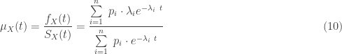
The failure rate (also called the hazard rate) can be interpreted as the rate of failure at the instant right after the life has survived to age 


where 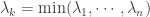
To see why 


Though not discussed here, several distributional quantities that are based on moments can be calculated, properties such as skewness and kurtosis, using the moments obtained in 
_______________________________________________________________________________________________
The Hypoexponential Density Function
The remainder of the post discusses the basic properties of the hypoexponential distribution. We first examine the probability density function of a hypoexponential distribution. Since such a distribution is an independent sum, the concept of convolution can be used. The following example show how it is done for the hypoexponential distribution with 2 phases. It turns out that the density function in general has a nice form.
Example 1
Suppose the rate parameters are 


The integral for the density function is:
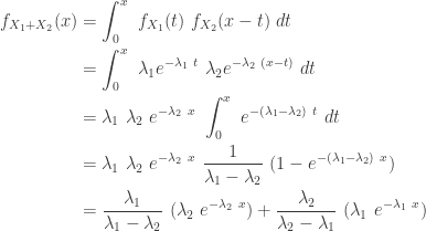
Note that the density 

Example 2
Suppose that the hypoexponential distribution has three phases. The parameters of the three phases are 
The idea is to apply the convolution of the density obtained in Example 1 and the exponential density 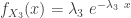
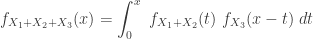
The result of the integral is:
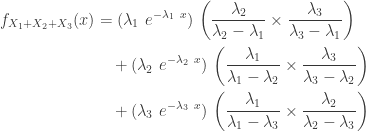
The density function 
Now, the general form of the density function for a hypoexponential density function.

where the weight 
The density function in the general case of
_______________________________________________________________________________________________
More Hypoexponential Properties
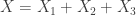
As before, the hypoexponential random variable is the sum 
![\displaystyle E[X]=\frac{1}{\lambda_1}+\frac{1}{\lambda_2}+\cdots+\frac{1}{\lambda_2} \ \ \ \ \ \ \ \ \ \ \ \ \ \ \ \ \ \ \ \ \ \ \ \ \ \ \ \ \ \ \ \ \ \ \ \ \ \ \ \ \ \ \ \ \ \ \ \ \ \ \ (13)](https://s0.wp.com/latex.php?latex=%5Cdisplaystyle+E%5BX%5D%3D%5Cfrac%7B1%7D%7B%5Clambda_1%7D%2B%5Cfrac%7B1%7D%7B%5Clambda_2%7D%2B%5Ccdots%2B%5Cfrac%7B1%7D%7B%5Clambda_2%7D+%5C+%5C+%5C+%5C+%5C+%5C+%5C+%5C+%5C+%5C+%5C+%5C+%5C+%5C+%5C+%5C+%5C+%5C+%5C+%5C+%5C+%5C+%5C+%5C+%5C+%5C+%5C+%5C+%5C+%5C+%5C+%5C+%5C+%5C+%5C+%5C+%5C+%5C+%5C+%5C+%5C+%5C+%5C+%5C+%5C+%5C+%5C+%5C+%5C+%5C+%5C+%2813%29&bg=ffffff&fg=333333&s=0&c=20201002)
![\displaystyle Var[X]=\frac{1}{\lambda_1^2}+\frac{1}{\lambda_2^2}+\cdots+\frac{1}{\lambda_2^2} \ \ \ \ \ \ \ \ \ \ \ \ \ \ \ \ \ \ \ \ \ \ \ \ \ \ \ \ \ \ \ \ \ \ \ \ \ \ \ \ \ \ \ \ \ \ \ \ (14)](https://s0.wp.com/latex.php?latex=%5Cdisplaystyle+Var%5BX%5D%3D%5Cfrac%7B1%7D%7B%5Clambda_1%5E2%7D%2B%5Cfrac%7B1%7D%7B%5Clambda_2%5E2%7D%2B%5Ccdots%2B%5Cfrac%7B1%7D%7B%5Clambda_2%5E2%7D+%5C+%5C+%5C+%5C+%5C+%5C+%5C+%5C+%5C+%5C+%5C+%5C+%5C+%5C+%5C+%5C+%5C+%5C+%5C+%5C+%5C+%5C+%5C+%5C+%5C+%5C+%5C+%5C+%5C+%5C+%5C+%5C+%5C+%5C+%5C+%5C+%5C+%5C+%5C+%5C+%5C+%5C+%5C+%5C+%5C+%5C+%5C+%5C+%2814%29&bg=ffffff&fg=333333&s=0&c=20201002)
The coefficient of variation is the ratio of the standard deviation to the mean. For the exponential distribution, the coefficient of variation is always 1. For the hypoexponential distribution, the coefficient of variation is always less than 1. The following is the square of the coefficient of variation for a hypoexponential random variable.
![\displaystyle \text{CV}^2=\frac{Var[X]}{E[X]^2}=\frac{\frac{1}{\lambda_1^2}+\frac{1}{\lambda_2^2}+\cdots+\frac{1}{\lambda_2^2}}{\biggl(\frac{1}{\lambda_1}+\frac{1}{\lambda_2}+\cdots+\frac{1}{\lambda_2}\biggr)^2}<1 \ \ \ \ \ \ \ \ \ \ \ \ \ \ \ \ \ \ \ \ \ \ \ \ \ \ \ \ (15)](https://s0.wp.com/latex.php?latex=%5Cdisplaystyle+%5Ctext%7BCV%7D%5E2%3D%5Cfrac%7BVar%5BX%5D%7D%7BE%5BX%5D%5E2%7D%3D%5Cfrac%7B%5Cfrac%7B1%7D%7B%5Clambda_1%5E2%7D%2B%5Cfrac%7B1%7D%7B%5Clambda_2%5E2%7D%2B%5Ccdots%2B%5Cfrac%7B1%7D%7B%5Clambda_2%5E2%7D%7D%7B%5Cbiggl%28%5Cfrac%7B1%7D%7B%5Clambda_1%7D%2B%5Cfrac%7B1%7D%7B%5Clambda_2%7D%2B%5Ccdots%2B%5Cfrac%7B1%7D%7B%5Clambda_2%7D%5Cbiggr%29%5E2%7D%3C1+%5C+%5C+%5C+%5C+%5C+%5C+%5C+%5C+%5C+%5C+%5C+%5C+%5C+%5C+%5C+%5C+%5C+%5C+%5C+%5C+%5C+%5C+%5C+%5C+%5C+%5C+%5C+%5C+%2815%29&bg=ffffff&fg=333333&s=0&c=20201002)
![\displaystyle \text{CV}=\frac{\sigma_X}{E[X]}<1 \ \ \ \ \ \ \ \ \ \ \ \ \ \ \ \ \ \ \ \ \ \ \ \ \ \ \ \ \ \ \ \ \ \ \ \ \ \ \ \ \ \ \ \ \ \ \ \ \ \ \ \ \ \ \ \ \ \ \ \ \ \ \ \ \ \ (16)](https://s0.wp.com/latex.php?latex=%5Cdisplaystyle+%5Ctext%7BCV%7D%3D%5Cfrac%7B%5Csigma_X%7D%7BE%5BX%5D%7D%3C1+%5C+%5C+%5C+%5C+%5C+%5C+%5C+%5C+%5C+%5C+%5C+%5C+%5C+%5C+%5C+%5C+%5C+%5C+%5C+%5C+%5C+%5C+%5C+%5C+%5C+%5C+%5C+%5C+%5C+%5C+%5C+%5C+%5C+%5C+%5C+%5C+%5C+%5C+%5C+%5C+%5C+%5C+%5C+%5C+%5C+%5C+%5C+%5C+%5C+%5C+%5C+%5C+%5C+%5C+%5C+%5C+%5C+%5C+%5C+%5C+%5C+%5C+%5C+%5C+%5C+%5C+%2816%29&bg=ffffff&fg=333333&s=0&c=20201002)
Note that the quantity in the denominator in 


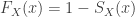
The survival function for the hypoexponential distribution has the following form:

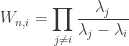
where the weights 

With the density function in
The following is the failure rate of the hypoexponential distribution.
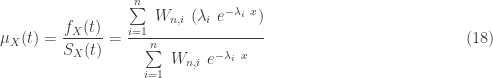
The hypoexponential failure rate is obviously not a constant rate since only the exponential distribution has constant failure rate. However, as the system reaches high ages, the failure rate approaches that of the smallest exponential rate parameters that define the hypoexponential distribution. The same observation is made above in

where 


_______________________________________________________________________________________________


Sorry for my poor english. Thanks for the article, i now finally understand the hypoexponential distribution better and find it vividly explained. For me, however, remains the failure rate in the hyperexponential distribution when needed for serial phases. This formula for failure rates i believe is only relative to the beginning of the “experiment”, and not over the “whole time”, but I am unsure.
LikeLike
Pingback: A catalog of parametric severity models | Topics in Actuarial Modeling
Pingback: Practice Problem Set 5 – Exercises for Severity Models « Practice Problems in Actuarial Modeling