Transformed gamma distribution

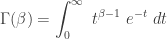
The previous post opens up a discussion on generating distributions by raising an existing distribution to a power. The previous post focuses on the example of raising an exponential distribution to a power. This post focuses on the distributions generated by raising a gamma distribution to a power.

Raising to a Power

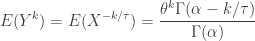
Let $X$ be a random variable. Let $\tau$ be a positive constant. The random variables $Y=X^{1/\tau}$ , $Y=X^{-1}$ and $Y=X^{-1/\tau}$ are called transformed, inverse and inverse transformed, respectively.

Let $f_X(x)$ , $F_X(x)$ and $S_X(x)=1-F_X(x)$ be the probability density function (PDF), the cumulative distribution function (CDF) and the survival function of the random variable $X$ (the base distribution). The following derivation seeks to express the CDFs of the “transformed” variables in terms of the base CDF $F_X(x)$ .

$Y=X^{1/\tau}$

(Transformed)

$\displaystyle \begin{aligned} F_Y(y)&=P(Y \le y) \\&=P(X^{1/\tau} \le y) \\&=P(X \le y^\tau) \\&=F_X(y^\tau) \end{aligned}$

$Y=X^{-1}$ (Inverse):
$\displaystyle \begin{aligned} F_Y(y)&=P(Y \le y) \\&=P(X^{-1} \le y) \\&=P(X \ge y^{-1}) \\&=S_X(y^{-1})=1-F_X(y^{-1}) \end{aligned}$

$Y=X^{-1/\tau}$ (Inverse Transformed):
$\displaystyle \begin{aligned} F_Y(y)&=P(Y \le y) \\&=P(X^{-1/\tau} \le y)\\&=P(X^{-1} \le y^\tau) \\&=P(X \ge y^{-\tau)} \\&=S_X(y^{-\tau})=1-F_X(y^{-\tau}) \end{aligned}$

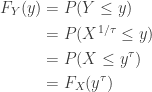
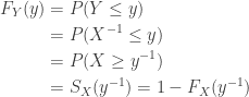
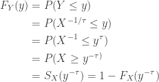
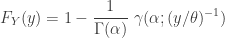
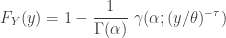
Gamma CDF

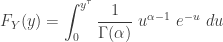
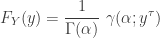
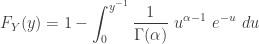
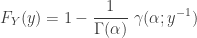
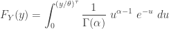
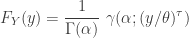
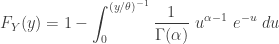
Unlike the exponential distribution, the CDF of the gamma distribution does not have a closed form. Suppose that $X$ is a random variable that has a gamma distribution with shape parameter $\alpha$ and scale parameter $\theta$ . The following is the expression of the gamma CDF.

$\displaystyle F_X(x)=\int_0^x \frac{1}{\Gamma(\alpha)} \ \frac{1}{\theta^\alpha} \ t^{\alpha-1} \ e^{- t/\theta} \ dt \ \ \ \ \ \ \ \ \ x>0$

By a change of variable, the CDF can be expressed as the following integral.

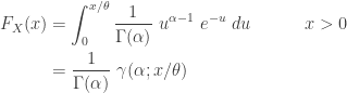
$\displaystyle \begin{aligned} F_X(x)&=\int_0^{x/\theta} \frac{1}{\Gamma(\alpha)} \ u^{\alpha-1} \ e^{- u} \ du \ \ \ \ \ \ \ \ \ x>0 \\&=\frac{1}{\Gamma(\alpha)} \ \gamma(\alpha; x/\theta) \end{aligned}$

Note that $\Gamma(\cdot)$ and $\gamma(\beta;\cdot)$ are the gamma function and incomplete gamma function, respectively, defined as follows.

$\displaystyle \Gamma(\beta)=\int_0^\infty \ t^{\beta-1} \ e^{- t} \ dt$

$\displaystyle \gamma(\beta; w)=\int_0^w \ t^{\beta-1} \ e^{- t} \ dt$

The CDF $F_X(x)$ can be evaluated numerically using software. When the gamma distribution is raised to a power, the resulting CDF will be defined as a function of $F_X(x)$ .

“Transformed” Gamma CDFs

The CDF of the “transformed” gamma distributions does not have a closed form. Thus the CDFs are to be defined based on an integral or the incomplete gamma function, shown in the preceding section. We still use the two-step approach – first deriving the CDF without the scale parameter and then add it at the end. Based on the two preceding sections, the following shows the CDFs of the three different cases.

Step 1. “Transformed” Gamma CDF (without scale parameter)


Transformed	$Y=X^{1 / \tau}$	$\tau >0$
	$F_Y(y)=F_X(y^\tau)$
	$\displaystyle F_Y(y)=\int_0^{y^\tau} \frac{1}{\Gamma(\alpha)} \ u^{\alpha-1} \ e^{- u} \ du$	$y >0$
	$\displaystyle F_Y(y)=\frac{1}{\Gamma(\alpha)} \ \gamma(\alpha; y^\tau)$	$y >0$
Inverse	$Y=X^{1 / \tau}$	$\tau=-1$
	$F_Y(y)=S_X(y^{-1})=1-F_X(y^{-1})$
	$\displaystyle F_Y(y)=1-\int_0^{y^{-1}} \frac{1}{\Gamma(\alpha)} \ u^{\alpha-1} \ e^{- u} \ du$	$y >0$
	$\displaystyle F_Y(y)=1-\frac{1}{\Gamma(\alpha)} \ \gamma(\alpha; y^{-1})$	$y >0$
Inverse Transformed	$Y=X^{-1 / \tau}$	$\tau >0$
	$F_Y(y)=S_X(y^{-\tau})=1-F_X(y^{-\tau})$
	$\displaystyle F_Y(y)=1-\int_0^{y^{-\tau}} \frac{1}{\Gamma(\alpha)} \ u^{\alpha-1} \ e^{- u} \ du$	$y >0$
	$\displaystyle F_Y(y)=1-\frac{1}{\Gamma(\alpha)} \ \gamma(\alpha; y^{-\tau})$	$y >0$

Step 2. “Transformed” Gamma CDF (with scale parameter)


Transformed	$Y=X^{1 / \tau}$	$\tau >0$
	$\displaystyle F_Y(y)=\int_0^{(y/\theta)^\tau} \frac{1}{\Gamma(\alpha)} \ u^{\alpha-1} \ e^{- u} \ du$	$y >0$
	$\displaystyle F_Y(y)=\frac{1}{\Gamma(\alpha)} \ \gamma(\alpha; (y/\theta)^\tau)$	$y >0$
Inverse	$Y=X^{1 / \tau}$	$\tau=-1$
	$\displaystyle F_Y(y)=1-\int_0^{(y/\theta)^{-1}} \frac{1}{\Gamma(\alpha)} \ u^{\alpha-1} \ e^{- u} \ du$	$y >0$
	$\displaystyle F_Y(y)=1-\frac{1}{\Gamma(\alpha)} \ \gamma(\alpha; (y/\theta)^{-1})$	$y >0$
Inverse Transformed	$Y=X^{-1 / \tau}$	$\tau >0$
	$\displaystyle F_Y(y)=1-\int_0^{(y/\theta)^{-\tau}} \frac{1}{\Gamma(\alpha)} \ u^{\alpha-1} \ e^{- u} \ du$	$y >0$
	$\displaystyle F_Y(y)=1-\frac{1}{\Gamma(\alpha)} \ \gamma(\alpha; (y/\theta)^{-\tau})$	$y >0$

The transformed gamma distribution and the inverse transformed gamma distribution are three-parameter distributions with $\tau$ being the shape parameter, $\theta$ being the scale parameter and $\tau$ being in the power to which the base gamma distribution is raised. The inverse gamma distribution has two parameters with $\theta$ being the scale parameter and $\alpha$ being shape parameter (the same two parameters in the base gamma distribution). Computation of these CDFs would require the use of software that can evaluate incomplete gamma function.

Another Way to Work with “Transformed” Gamma

The CDFs derived in the preceding section is a two-step approach – first raising a gamma distribution with scale parameter equals to 1 to a power and then adding a scale parameter. The end result gives CDFs that are a function of the incomplete gamma function. Calculating a CDF would require using a software that has the capability of evaluating incomplete gamma function (or evaluating an equivalent integral). If the software that is used does not have the incomplete gamma function but has gamma CDF (e.g. Excel), then there is another way of generating the “transformed” gamma CDF.

Observe that the CDFs in the last section are the results of raising a base gamma distribution with shape parameter $\alpha$ and $\theta^\tau$ (transformed), shape parameter $\alpha$ and $\theta^{-1}$ (inverse) and shape parameter $\alpha$ and $\theta^{-\tau}$ (inverse transformed). Based on this observation, we can evaluate the CDFs and the moments. This section shows how to evaluate CDFs using this approach. The next section shows how to evaluate the moments.

Transformed Gamma Distribution

Given a transformed gamma random variable $Y$ with parameters $\tau$ , $\alpha$ (shape) and $\theta$ (scale), know that $Y=X^{1/\tau}$ where $X$ gas a gamma distribution with parameters $\alpha$ (shape) and $\theta^\tau$ (scale). Then $F_Y(y)=F_X(y^\tau)$ such that $F_X(y^\tau)$ is evaluated using a software with the capability of evaluating gamma CDF (e.g. Excel).

Inverse Gamma Distribution

Given an inverse gamma random variable $Y$ with parameters $\tau$ and $\theta$ (scale), know that $Y=X^{-1}$ where $X$ gas a gamma distribution with parameters $\alpha$ (shape) and $\theta^{-1}$ (scale). Then $F_Y(y)=S_X(y^{-1})=1-F_X(y^{-1})$ such that $F_X(y^{-1})$ is evaluated using a software with the capability of evaluating gamma CDF (e.g. Excel).

Inverse Transformed Gamma Distribution

Given an inverse transformed gamma random variable $Y$ with parameters $\tau$ , $\alpha$ (shape) and $\theta$ (scale), know that $Y=X^{-1/\tau}$ where $X$ gas a gamma distribution with parameters $\alpha$ (shape) and $\theta^{-\tau}$ (scale). Then $F_Y(y)=S_X(y^{-\tau})=1-F_X(y^{-\tau})$ such that $F_X(y^{-\tau})$ is evaluated using a software with the capability of evaluating gamma CDF (e.g. Excel).

Example 1 below uses Excel to compute the transformed gamma CDF.

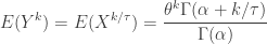
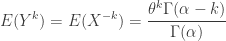
“Transformed” Gamma Moments

Following the idea in the preceding section, the moments for the “transformed” gamma moments can be derived using gamma moments with the appropriate parameters (see here for the gamma moments). The following table shows the results.

“Transformed Gamma Moments

	Base Gamma Parameters	Moments
Transformed	$\alpha$ and $\theta^\tau$	$\displaystyle E(Y^k)=E(X^{k/\tau})=\frac{\theta^k \Gamma(\alpha+k/\tau)}{\Gamma(\alpha)}$
		$k>- \alpha \ \tau$
Inverse	$\alpha$ and $\theta^{-1}$	$\displaystyle E(Y^k)=E(X^{-k})=\frac{\theta^k \Gamma(\alpha-k)}{\Gamma(\alpha)}$
		$k<\alpha$
Inverse Transformed	$\alpha$ and $\theta^{-\tau}$	$\displaystyle E(Y^k)=E(X^{-k/\tau})=\frac{\theta^k \Gamma(\alpha-k/\tau)}{\Gamma(\alpha)}$
		$k<\alpha \ \tau$

Note that the moments for the transformed gamma distribution exists for all positive $k$ . The moments for inverse gamma are limited (capped by the shape parameter $\alpha$ ). The moments for inverse transformed gamma are also limited, this time limited by both parameters. The computation for these moments is usually done by software, except when the argument of the gamma function is a positive integer.

“Transformed” Gamma PDFs

Once the CDFs are known, the PDFs are derived by taking derivative. The following table gives the three PDFs.

“Transformed” Gamma PDFs


Transformed	$\displaystyle f_Y(y)=\frac{\tau}{\Gamma(\alpha)} \ \biggl( \frac{y}{\theta} \biggr)^{\tau \alpha} \ \frac{1}{y} \ \exp(-(y/\theta)^\tau)$	$y>0$
	$\text{ }$
Inverse	$\displaystyle f_Y(y)=\frac{1}{\Gamma(\alpha)} \ \biggl( \frac{\theta}{y} \biggr)^{\alpha} \ \frac{1}{y} \ \exp(-\theta/y)$	$y>0$
	$\text{ }$
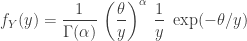Inverse Transformed	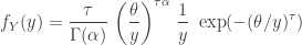$\displaystyle f_Y(y)=\frac{\tau}{\Gamma(\alpha)} \ \biggl( \frac{\theta}{y} \biggr)^{\tau \alpha} \ \frac{1}{y} \ \exp(-(\theta/y)^\tau)$	$y>0$

Each PDF is obtained by taking derivative of the integral for the corresponding CDF.

Example

The post is concluded with one example demonstrating the calculation for CDF and percentiles using the gamma distribution function in Excel.

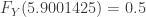
Example 1
The size of a collision claim from a large pool of auto insurance policies has a transformed gamma distribution with parameters $\tau=2$ , $\alpha=2.5$ and $\theta=4$ . Determine the following.

The probability that a randomly selected claim is greater than than 6.75.
The probability that a randomly selected claim is between 4.25 and 8.25.
The median size of a claim from this pool of insurance policies.
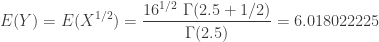
The mean and variance of a claim from this pool of insurance policies.
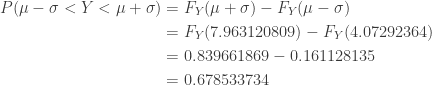
The probability that a randomly selected claim is within one standard deviation of the mean claim size.
The probability that a randomly selected claim is within two standard deviations of the mean claim size.

Since $\tau=2$ , this is a transformed gamma distribution. There are two ways to get a handle on this distribution. One way is to plug in the three parameters $\tau=2$ , $\alpha=2.5$ and $\theta=4$ into the transformed gamma CDF (in the table Step 2. “Transformed” Gamma CDF (with scale parameter)). This would require using a software that can evaluate the incomplete gamma function or its equivalent integrals. The other way is to know that this distribution is the result of raising the gamma distribution with shape parameter $\alpha=2.5$ and scale parameter $4^2=16$ to the power of 1/2. We take the latter approach.

In Excel, =GAMMA.DIST(A1,B1,C1,TRUE) is the function that produces the gamma CDF $F_X(x)$ , assuming that the value $x$ is in cell A1, the shape parameter is in cell B1 and the scale parameter is in cell C1. When the last parameter is TRUE, it gives the CDF. If it is FALSE, it gives the PDF. For example, =GAMMA.DIST(2.5, 2, 1, TRUE) gives the value of 0.712702505.

The transformed gamma distribution in question (random variable $Y$ ) is the result of raising gamma $\alpha=2.5$ and scale parameter 16 (random variable $X$ ) to 1/2. Thus the CDF $F_Y(y)$ is obtained from evaluating the gamma CDF $F_X(y^2)$ , which is =GAMMA.DIST( $y^2$ , 2.5, 16, TRUE). As a result, the following gives the answers for the first two bullet points.

$P(Y>6.75)=1-F_X(6.75)=1-0.663=0.337$

$6.75^2$

$P(4.25 \le Y \le 8.25)=F_X(8.25)-F_X(4.25)=0.8696-0.1876=0.6820$

The median or other percentiles of transformed gamma distribution are obtained by a trial and error approach, i.e. by plugging in values of $y$ into the gamma CDF =GAMMA.DIST( $y^2$ , 2.5, 16, TRUE). After performing the trial and error process, we see that $F_Y(5.9001425)=0.5$ and $F_Y(5.9101425)=0.502020715$ . Thus we take the median to be 5.9. So the median size of a claim is around 5.9.

Computation of the moments of a gamma distribution requires the evaluation of the gamma function $\Gamma(\cdot)$ . Excel does not have an explicit function for gamma function. Since $\Gamma(\cdot)$ is in the gamma PDF, we can derive the gamma function from the gamma PDF in Excel =GAMMA.DIST(1, a, 1, FALSE). The value of this gamma PDF is $e^{-1}/\Gamma(a)$ . This the value of $\Gamma(a)$ is $e^{-1}$ divided by the value of this gamma PDF value. For example, the following Excel formulas give $\Gamma(5)$ and $\Gamma(2.5)$ .

=EXP(-1)/GAMMA.DIST(1, 2.5, 1, FALSE) = 1.329340388

The moments $E(Y^k)$ is $E(X^{k/2})$ . Based on the results in the section on “Transformed” gamma moments, the following gives the mean and variance.

$\displaystyle E(Y)=E(X^{1/2})=\frac{16^{1/2} \ \Gamma(2.5+1/2)}{\Gamma(2.5)}=6.018022225$

$\displaystyle E(Y^2)=E(X)=2.5 \cdot 16=40$

$Var(Y)=40-6.018022225^2=3.783408505$

$\sigma_Y=3.783408505^{0.5}=1.945098585$

The following gives the probability of a claim within one or two standard deviations of the mean.

$\displaystyle \begin{aligned} P(\mu-\sigma<Y<\mu+\sigma)&=F_Y(\mu+\sigma)-F_Y(\mu-\sigma) \\&=F_Y(7.963120809)-F_Y(4.07292364) \\&=0.839661869-0.161128135 \\&=0.678533734 \end{aligned}$

$\displaystyle \begin{aligned} P(\mu-2 \sigma<Y<\mu+2 \sigma)&=F_Y(\mu+2 \sigma)-F_Y(\mu-2 \sigma) \\&=F_Y(9.908219394)-F_Y(2.127825055) \\&=0.968750102-0.010491099 \\&=0.958259003 \end{aligned}$

$\text{ }$

6 thoughts on “Transformed gamma distribution”

Pingback: Transformed exponential distributions | Topics in Actuarial Modeling
Pingback: Gamma Function and Gamma Distribution – Daniel Ma
Pingback: Transformed Pareto distribution | Topics in Actuarial Modeling
Pingback: The Gamma Function | A Blog on Probability and Statistics
Pingback: A catalog of parametric severity models | Topics in Actuarial Modeling
Boris Polanco says:

on June 6, 2018 at 3:40 am

Hi Dan Ma, nice explanation. Just could you explain me the case when is considered the transformation of the gamma with scale parameter included? I cannot understand why the scale parameter is also to the power tau. Also with the inverse and the inverse transform.

best Regards and good forum very helpful!!

LikeLike

Topics in Actuarial Modeling

exploring the mathematical and statistical aspects of actuarial science

Transformed gamma distribution

6 thoughts on “Transformed gamma distribution”

Leave a comment Cancel reply

Share this:

6 thoughts on “Transformed gamma distribution”

Leave a comment Cancel reply