The Chi-Squared Distribution, Part 3c

This post is part of a series of posts on chi-squared distribution. Three of the posts, this one and the previous two posts, deal with inference involving categorical variables. This post discusses the chi-squared test of independence. The previous two posts are on chi-squared goodness of fit test (part 3a) and on chi-squared test of homogeneity (part 3b).

The first post in the series is an introduction on chi-squared distribution. The second post is on several inference procedures that are based on chi-squared distribution that deal with quantitative measurements.

The 3-part discussion in part 3a, part 3b and part 3c are three different interpretations of the chi-squared test. Refer to the other two posts for the other two interpretations. We also make remarks below on the three chi-squared tests.

_______________________________________________________________________________________________

Two-Way Tables

In certain analysis of count data of categorical variables, we are interested in whether two categorical variables are associated with one another (or are related to one another). In such analysis, it is useful to represent the count data in a two-way table or contingency table. The following gives two examples using survival data in the ocean liner Titanic.

Table 1 – Survival status of the passengers in the Titanic by gender group


Table 2 – Survival status of the passengers in the Titanic by passenger class

Table 1 shows the count data for the survival status (survived or not survived) and gender of the passengers in the one and only voyage of the passenger liner Titanic. Table 2 shows the survival status and the passenger class of the passengers of Titanic. Both tables are contingency tables or two-way since each table relates two categorical variables – survival status and gender in Table 1 and survival status and passenger class in Table 2. Each table summarizes the categorical data by counting the number of observations that fall into each group for the two variables. For example, Table 1 shows that there were 304 women passengers who survived. In both tables, the survival status is the row variable. The column variable is gender (Table 1) or passenger class (Table 2).

It is clear from both tables that most of the deaths were either men or third class passengers. This observation is not surprising because of the mentality of “Women and Children First” and the fact that first class passengers were better treated than the other classes. Thus we can say that there is an association between gender and survival and there is an association between passenger class and survival in the sinking of Titanic. More specifically, the survival rates for women and children were much higher than for men and the survival rates for first class passenger was much higher than for the other two classes.

When a study measures two categorical variables on each individual in a random sample, the results can be summarized in a two-way table, which can then be used for studying the relationship between the two variables. As a first step, joint distribution, marginal distributions and conditional distributions are analyzed. Table 1 is analyzed in here. Table 2 is analyzed here. Though the Titanic survival data show a clear association between survival and gender (and passenger class), the discussion of the Titanic survival data in these two previous posts is still very useful. These two posts demonstrate how to analyze the relationship between two categorical variables by looking at the marginal distributions and conditional distributions.

This post goes one step further by analyzing the relationship in a two-way table using the chi-squared test. The method discussed here is called the chi-squared test of independence, in other words, the test determines whether there is a relationship between the two categorical variables displayed in a two-way table.

_______________________________________________________________________________________________

Test of Independence

We demonstrate the test of independence by working through the following example (Example 1). When describing how the method works in general, the two-way table has rows and columns (not including the total row and the total column).

Example 1
The following table shows the smoking status and the level of education of residents (aged 25 or over) of a medium size city on the East coast of the United States based on a survey conducted on a random sample of 1,078 adults aged 25 or older.

Table 3 – Smoking Status and Level of Education

The researcher is interested in finding out whether smoking status is associated with the level of education among the adults in this city. Do the data in Table 3 provide sufficient evidence to indicate that smoking status is affected by the level of education among the adults in this city?

The two categorical variables in this example are smoking status (current, former and never smoker) and level of education (the 4 categories listed in the columns in Table 3). The researcher views level of education as an explanatory variable and smoking status as the response variable. Table 3 has 3 rows and 4 columns. Thus there are 12 cells in the table. It is helpful to obtain the total for each row and the total for each column.

Table 3a – Smoking Status and Level of Education

The null hypothesis in a two-way table is the statement that there is no association between the row variable and the column variable, i.e., the row variable and the column variable are independent. The alternative hypothesis states that there is an association between the two variables. For Table 3, the null hypothesis is that there is no association between the smoking status and the level of education among the adults in this city.

In Table 3 or 3a, each column is a distribution of smoking status (for each level of education). Another way to state the null hypothesis is that the distributions of the smoking status are the same across the four levels of educations. The alternative hypothesis is that the distributions are not the same.

Our goal is to use the chi-squared statistic to evaluate the data in the two-way table. The chi-squared statistic is based the squared difference between the observed counts in Table 3a and the expected counts derived from assuming the null hypothesis. The following shows how to calculate the expected count for each cell assuming the null hypothesis.

The in the denominator is the total number of observations in the two-way table. For Table 3a, 1078. For the cell of “Current Smoker” and “Did not Finish High School”, the expected count would be 476 x 401 / 1078 = 177.06. The other expected counts are calculated accordingly and are shown in Table 3b with the expected counts in parentheses.

Table 3b – Smoking Status and Level of Education

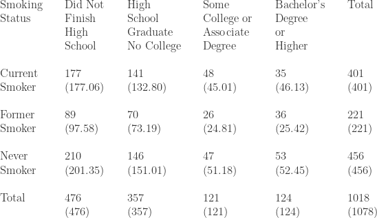
How do we know if the formula for the expected cell count is correct? Look at the right margin of Table 3a or 3b (Total column). The counts 401, 221 and 456 as percentages of the total 1078 are 37.20%, 20.50% and 42.30%. If the null hypothesis that there is no relation between level of education and smoking status is true, we would expect these overall percentages to apply to each level of education. For example, there are 476 adults in the sample who did not complete high school. We would expect 37.20% of them to be current smokers, 20.50% of them to be former smokers and 42.30% of them to be never smokers if indeed smoker status is not affected by level of education. In particular, 37.20% x 476 = 177.072 (the same as 177.06 ignoring the rounding difference). Note that 37.20% is the fraction 401/1078. As a result, 37.20% x 476 is identical to 476 x 401 / 1078. This confirms the formula stated above.

We now compute the chi-squared statistic. From a two-way table perspective, the chi-squared statistic is a measure of how much the observed cell counts deviate from the expected cell counts. The following formula makes this idea more explicit.

The sum in the formula is over all cells in the 2-way table where is the number of rows and is the number of columns. Note that the calculation of the chi-squared statistic is based on the expected counts discussed above. The expected counts are based on the assumption of the null hypothesis. Thus the chi-squared statistic is based on assuming the null hypothesis.

When the observed counts and the expected counts are very different, the value of the chi-squared statistic will be large. Thus large values of the chi-squared statistic provide evidence against the null hypothesis. In order to evaluate the observed data as captured in the chi-squared statistic, we need to have information about the sampling distribution of the chi-squared statistic as defined here.

If the null hypothesis is true, the chi-squared statistic defined above has an approximate chi-squared distribution with degrees of freedom. Recall that is the number of rows and is the number of columns in the two-way table (not counting the total row and total column).

Thus the null hypothesis is rejected if the value of the chi-squared statistic exceeds the critical value, which is the upper tail in the chi-squared distribution (with the appropriate df) of area (i.e. level of significance). The p-value approach can also be used. The p-value is the probability that the chi-squared random variable under the assumption of is more extreme than the observed chi-squared statistic.

The calculation of the chi-squared statistic for Table 3b is best done in software. Performing the calculation in Excel gives 9.62834 with df = (3-1) x (4-1) = 6. At level of significance 0.05, the critical value is 12.59. Thus the chi-squared statistic is not large enough to reject the null hypothesis. So the sample results do not provide enough evidence to conclude that smoking status is affected by level of education.

The p-value is 0.1412. Since this is a large p-value, we have the same conclusion that there is not sufficient evidence to reject the null hypothesis.

Both the critical value and the p-value are evaluated using the following functions in Excel.

Critical Value = CHISQ.INV.RT(level of significance, df)
p-value = 1 – CHISQ.DIST(test statistic, df, TRUE)

_______________________________________________________________________________________________

Another Example

Example 2
A researcher wanted to determine whether race/ethnicity is associated with political affiliations among the residents in a medium size city in the Eastern United States. The following table represents the ethnicity and the political affiliations from a random sample of adults in this city.

Table 4 – Race/Ethnicity and Political Affiliations

Use the chi-squared test as described above to test whether political affiliation is affected by race and ethnicity.

The following table show the calculation of the expected counts (in parentheses) and the total counts.

Table 4a – Race/Ethnicity and Political Affiliations

The value of the chi-squared statistic, computed in Excel, is 18.35, with df = (3-1) x (4-1) = 6. The critical value at level of significance 0.01 is 16.81. Thus we reject the null hypothesis that there is no relation between race/ethnicity and political party affiliation. The two-way table provides evidence that political affiliation is affected by race/ethnicity.

The p-value is 0.0054. This is the probability of obtaining a calculated value of the chi-squared statistic that is 18.35 or greater (assuming the null hypothesis). Since this probability is so small, it is unlikely that the large chi-squared value of 18.35 occurred by chance alone.

One interesting point that should be made is that the chi-squared test of independence does not provide insight into the nature of the association between the row variable and the column variable. To help clarify the association, it will be helpful to conduct analysis using marginal distributions and conditional distributions (as discussed here and here for the Titanic survival data).

_______________________________________________________________________________________________

Remarks

Some students may confuse the test of independence discussed here with the chi-squared test of homogeneity discussed in this previous post. Both tests can be used to test whether the distributions of the row variable are the same across the columns.

Bear in mind that the test of independence as discussed here is a way test whether two categorical variables (one on the rows and one on the columns) are associated with one another in a population. We discuss two examples here – level of education and smoking status in Example 1 and race/ethnicity and political affiliation in Example 2. In both cases, we want to see if one of the variable is affected by the other variable.

The test of homogeneity is a way to test whether two or more subgroups in a population follow the same distribution of a categorical variable. For example, do adults with different educational attainment levels have the same proportions of current smokers/former smokers/never smokers? For example, do adults in different racial groups have different proportions of independents, Democrats and Republicans?

Now the examples cited for the test of homogeneity seem to be the same examples we work for the test of independence. However, the two tests are indeed different. The difference is subtle. The difference is basically in the way the study is designed.

For the test of independence to be used, the observational units are collected at random from a population and two categorical variables are observed for each unit. Hence the results will be summarized in a two-way table. For the test of homogeneity, the data are collected by random sampling from each subgroup separately. If Example 2 is to use a test of homogeneity, the study would have to sample each racial group separately (say 1000 white, 1000 blacks and so on). Then we compare the proportions of party affiliations across racial group. For Example 2 to work as a test of independence as discussed here, the study would have to observe a random sample of adults and observe the race/ethnicity and party affiliation of each unit.

Another chi-squared test is called the goodness-of-fit test, discussed here. This test is a way of testing whether a set of observed categorical dataset come from a hypothesized distribution (e.g. Poison distribution).

All three tests use the same chi-squared statistic, but they are not the same test.

_______________________________________________________________________________________________

Reference

1. Moore D. S., McCabe G. P., Craig B. A., Introduction to the Practice of Statistics, 7th ed., W. H. Freeman and Company, New York, 2012
2. Wackerly D. D., Mendenhall III W., Scheaffer R. L.,Mathematical Statistics with Applications, Thomson Learning, Inc, California, 2008

_______________________________________________________________________________________________