
The notion of mixtures is discussed in this previous post. Many probability distributions useful for actuarial modeling are mixture distributions. The previous post touches on some examples – negative binomial distribution (a Poisson-Gamma mixture), Pareto distribution (an exponential-gamma mixture) and the normal-normal mixture. In this post we present additional examples. We discuss the following examples.
- Poisson-Gamma mixture = Negative Binomial.
- Normal-Normal mixture = Normal.
- Exponential-Gamma mixture = Pareto.
- Exponential-Inverse Gamma mixture = Pareto.
- Gamma-Gamma mixture = Generalized Pareto.
- Weibull-Exponential mixture = Loglogistic.
- Gamma-Geometric mixture = Exponential.
- Normal-Gamma mixture = Student t.
The first three examples are discussed in the previous post. We discuss the remaining examples in this post.
The Pareto Family
Examples 3 and 4 show that Pareto distributions are mixtures of exponential distributions with either gamma or inverse gamma mixing weights. In Example 3, 

As a mixture, Example 5 is like Example 3, except that it is a gamma-gamma mixture resulting in a generalized Pareto distribution. Example 3 has been discussed in the previous post. We now discuss Example 4 and Example 5.
Example 4. Suppose that
Further suppose that the random parameter 


The following gives the cumulative distribution function (CDF) and survival function of the conditional random variable
The random parameter
![\displaystyle g(\theta)=\frac{1}{\Gamma(\alpha)} \ \biggl[\frac{\beta}{\theta}\biggr]^\alpha \ \frac{1}{\theta} \ e^{-\frac{\beta}{ \theta}} \ \ \ \ \ \theta>0](https://s0.wp.com/latex.php?latex=%5Cdisplaystyle+g%28%5Ctheta%29%3D%5Cfrac%7B1%7D%7B%5CGamma%28%5Calpha%29%7D+%5C+%5Cbiggl%5B%5Cfrac%7B%5Cbeta%7D%7B%5Ctheta%7D%5Cbiggr%5D%5E%5Calpha+%5C+%5Cfrac%7B1%7D%7B%5Ctheta%7D+%5C+e%5E%7B-%5Cfrac%7B%5Cbeta%7D%7B+%5Ctheta%7D%7D+%5C+%5C+%5C+%5C+%5C+%5Ctheta%3E0&bg=ffffff&fg=333333&s=0&c=20201002)
We show that the unconditional survival function for
![\displaystyle \begin{aligned} S(x)&=\int_0^\infty S(x \lvert \theta) \ g(\theta) \ d \theta \\&=\int_0^\infty e^{- x/\theta} \ \frac{1}{\Gamma(\alpha)} \ \biggl[\frac{\beta}{\theta}\biggr]^\alpha \ \frac{1}{\theta} \ e^{-\beta / \theta} \ d \theta \\&=\int_0^\infty \frac{1}{\Gamma(\alpha)} \ \biggl[\frac{\beta}{\theta}\biggr]^\alpha \ \frac{1}{\theta} \ e^{-(x+\beta) / \theta} \ d \theta \\&=\frac{\beta^\alpha}{(x+\beta)^\alpha} \ \int_0^\infty \frac{1}{\Gamma(\alpha)} \ \biggl[\frac{x+\beta}{\theta}\biggr]^\alpha \ \frac{1}{\theta} \ e^{-(x+\beta) / \theta} \ d \theta \\&=\biggl(\frac{\beta}{x+\beta} \biggr)^\alpha \end{aligned}](https://s0.wp.com/latex.php?latex=%5Cdisplaystyle+%5Cbegin%7Baligned%7D+S%28x%29%26%3D%5Cint_0%5E%5Cinfty+S%28x+%5Clvert+%5Ctheta%29+%5C+g%28%5Ctheta%29+%5C+d+%5Ctheta+%5C%5C%26%3D%5Cint_0%5E%5Cinfty+e%5E%7B-+x%2F%5Ctheta%7D+%5C+%5Cfrac%7B1%7D%7B%5CGamma%28%5Calpha%29%7D+%5C+%5Cbiggl%5B%5Cfrac%7B%5Cbeta%7D%7B%5Ctheta%7D%5Cbiggr%5D%5E%5Calpha+%5C+%5Cfrac%7B1%7D%7B%5Ctheta%7D+%5C+e%5E%7B-%5Cbeta+%2F+%5Ctheta%7D+%5C+d+%5Ctheta+%5C%5C%26%3D%5Cint_0%5E%5Cinfty+%5Cfrac%7B1%7D%7B%5CGamma%28%5Calpha%29%7D+%5C+%5Cbiggl%5B%5Cfrac%7B%5Cbeta%7D%7B%5Ctheta%7D%5Cbiggr%5D%5E%5Calpha+%5C+%5Cfrac%7B1%7D%7B%5Ctheta%7D+%5C+e%5E%7B-%28x%2B%5Cbeta%29+%2F+%5Ctheta%7D+%5C+d+%5Ctheta+%5C%5C%26%3D%5Cfrac%7B%5Cbeta%5E%5Calpha%7D%7B%28x%2B%5Cbeta%29%5E%5Calpha%7D+%5C+%5Cint_0%5E%5Cinfty+%5Cfrac%7B1%7D%7B%5CGamma%28%5Calpha%29%7D+%5C+%5Cbiggl%5B%5Cfrac%7Bx%2B%5Cbeta%7D%7B%5Ctheta%7D%5Cbiggr%5D%5E%5Calpha+%5C+%5Cfrac%7B1%7D%7B%5Ctheta%7D+%5C+e%5E%7B-%28x%2B%5Cbeta%29+%2F+%5Ctheta%7D+%5C+d+%5Ctheta+%5C%5C%26%3D%5Cbiggl%28%5Cfrac%7B%5Cbeta%7D%7Bx%2B%5Cbeta%7D+%5Cbiggr%29%5E%5Calpha+%5Cend%7Baligned%7D&bg=ffffff&fg=333333&s=0&c=20201002)
Note that the the integrand in the last integral is a density function for an inverse gamma distribution. Thus the integral is 1 and can be eliminated. The result that remains is the survival function for a Pareto distribution with parameters
See here for further information on Pareto Type I Lomax distribution.
Example 5. Suppose that 
Conditional on 

The following is the density function of the random parameter
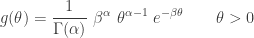
The following gives the unconditional density function for

Any distribution that has a density function described above is said to be a generalized Pareto distribution with the parameters

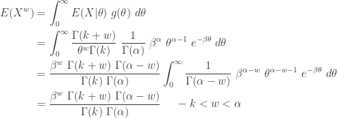
The moments can be easily derived for the generalized Pareto distribution but on a limited basis. Since it is a mixture distribution, the unconditional mean is the weighted average of the conditional means.
Note that 


When the parameter 
It turns out that the F distribution is also a special case of the generalized Pareto distribution. The F distribution with 


Another way to generate the F distribution is from taking a ratio of two chi-squared distributions (see Theorem 9 in this previous post). Of course, there is no need to use the explicit form of the density function of the F distribution. In a statistical application, the F distribution is accessed using tables or software.
The Loglogistic Distribution
The loglogistic distribution can be derived as a mixture of Weillbull distribution with exponential mixing weights.
Example 6. Suppose that 


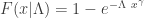


The following gives the conditional survival function for

The following gives the unconditional survival function and CDF of
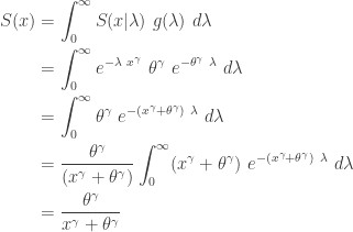
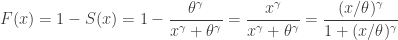
![\displaystyle f(x)=\frac{d}{dx} \biggl( \frac{x^\gamma}{x^\gamma+\theta^\gamma} \biggr)=\frac{\gamma \ (x/\theta)^\gamma}{x [1+(x/\theta)^\gamma]^2}](https://s0.wp.com/latex.php?latex=%5Cdisplaystyle+f%28x%29%3D%5Cfrac%7Bd%7D%7Bdx%7D+%5Cbiggl%28+%5Cfrac%7Bx%5E%5Cgamma%7D%7Bx%5E%5Cgamma%2B%5Ctheta%5E%5Cgamma%7D+%5Cbiggr%29%3D%5Cfrac%7B%5Cgamma+%5C+%28x%2F%5Ctheta%29%5E%5Cgamma%7D%7Bx+%5B1%2B%28x%2F%5Ctheta%29%5E%5Cgamma%5D%5E2%7D&bg=ffffff&fg=333333&s=0&c=20201002)
Any distribution that has any one of the above three distributional quantities is said to be a loglogistic distribution with shape parameter
One interesting point about loglogistic distribution that an inverse loglogistic distribution is another loglogistic distribution. Suppose that 


![\displaystyle \begin{aligned} P[Y \le y]&=P[\frac{1}{X} \le y] =P[X \ge y^{-1}] =\frac{\theta^\gamma}{y^{-\gamma}+\theta^\gamma} \\&=\frac{\theta^\gamma \ y^\gamma}{1+\theta^\gamma \ y^\gamma} \\&=\frac{y^\gamma}{(\theta^{-1})^\gamma+y^\gamma} \end{aligned}](https://s0.wp.com/latex.php?latex=%5Cdisplaystyle+%5Cbegin%7Baligned%7D+P%5BY+%5Cle+y%5D%26%3DP%5B%5Cfrac%7B1%7D%7BX%7D+%5Cle+y%5D+%3DP%5BX+%5Cge+y%5E%7B-1%7D%5D+%3D%5Cfrac%7B%5Ctheta%5E%5Cgamma%7D%7By%5E%7B-%5Cgamma%7D%2B%5Ctheta%5E%5Cgamma%7D+%5C%5C%26%3D%5Cfrac%7B%5Ctheta%5E%5Cgamma+%5C+y%5E%5Cgamma%7D%7B1%2B%5Ctheta%5E%5Cgamma+%5C+y%5E%5Cgamma%7D+%5C%5C%26%3D%5Cfrac%7By%5E%5Cgamma%7D%7B%28%5Ctheta%5E%7B-1%7D%29%5E%5Cgamma%2By%5E%5Cgamma%7D+%5Cend%7Baligned%7D&bg=ffffff&fg=333333&s=0&c=20201002)
The above is a survival function for the loglogistic distribution with the desired parameters. Thus there is no need to specially call out the inverse loglogistic distribution.
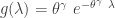
In order to find the mean and higher moments of the loglogistic distribution, we take the approach of identifying the conditional Weibull means and the weight these means by the exponential mixing weights. Note that the parameter 
![\displaystyle E[ (X \lvert \Lambda)^k]=\Gamma \biggl(1+\frac{k}{\gamma} \biggr) \Lambda^{-k/\gamma}](https://s0.wp.com/latex.php?latex=%5Cdisplaystyle+E%5B+%28X+%5Clvert+%5CLambda%29%5Ek%5D%3D%5CGamma+%5Cbiggl%281%2B%5Cfrac%7Bk%7D%7B%5Cgamma%7D+%5Cbiggr%29+%5CLambda%5E%7B-k%2F%5Cgamma%7D&bg=ffffff&fg=333333&s=0&c=20201002)
The following gives the unconditional
![\displaystyle \begin{aligned} E[X^k]&=\int_0^\infty E[ (X \lvert \Lambda)^k] \ g(\lambda) \ d \lambda \\&=\int_0^\infty \Gamma \biggl(1+\frac{k}{\gamma} \biggr) \lambda^{-k/\gamma} \ \theta^\gamma \ e^{-\theta^\gamma \ \lambda} \ d \lambda\\&=\Gamma \biggl(1+\frac{k}{\gamma} \biggr) \ \theta^\gamma \int_0^\infty \lambda^{-k/\gamma} \ e^{-\theta^\gamma \ \lambda} \ d \lambda \\&=\theta^k \ \Gamma \biggl(1+\frac{k}{\gamma} \biggr) \int_0^\infty t^{-k/\gamma} \ e^{-t} \ dt \ \ \text{ where } t=\theta^\gamma \lambda \\&=\theta^k \ \Gamma \biggl(1+\frac{k}{\gamma} \biggr) \int_0^\infty t^{[(\gamma-k)/\gamma]-1} \ e^{-t} \ dt \\&=\theta^k \ \Gamma \biggl(1+\frac{k}{\gamma} \biggr) \ \Gamma \biggl(1-\frac{k}{\gamma} \biggr) \ \ \ \ -\gamma<k<\gamma \end{aligned}](https://s0.wp.com/latex.php?latex=%5Cdisplaystyle+%5Cbegin%7Baligned%7D+E%5BX%5Ek%5D%26%3D%5Cint_0%5E%5Cinfty+E%5B+%28X+%5Clvert+%5CLambda%29%5Ek%5D+%5C+g%28%5Clambda%29+%5C+d+%5Clambda+%5C%5C%26%3D%5Cint_0%5E%5Cinfty+%5CGamma+%5Cbiggl%281%2B%5Cfrac%7Bk%7D%7B%5Cgamma%7D+%5Cbiggr%29+%5Clambda%5E%7B-k%2F%5Cgamma%7D+%5C+%5Ctheta%5E%5Cgamma+%5C+e%5E%7B-%5Ctheta%5E%5Cgamma+%5C+%5Clambda%7D+%5C+d+%5Clambda%5C%5C%26%3D%5CGamma+%5Cbiggl%281%2B%5Cfrac%7Bk%7D%7B%5Cgamma%7D+%5Cbiggr%29+%5C+%5Ctheta%5E%5Cgamma+%5Cint_0%5E%5Cinfty++%5Clambda%5E%7B-k%2F%5Cgamma%7D+%5C+e%5E%7B-%5Ctheta%5E%5Cgamma+%5C+%5Clambda%7D+%5C+d+%5Clambda+%5C%5C%26%3D%5Ctheta%5Ek+%5C+%5CGamma+%5Cbiggl%281%2B%5Cfrac%7Bk%7D%7B%5Cgamma%7D+%5Cbiggr%29++%5Cint_0%5E%5Cinfty++t%5E%7B-k%2F%5Cgamma%7D+%5C+e%5E%7B-t%7D+%5C+dt+%5C+%5C+%5Ctext%7B+where+%7D+t%3D%5Ctheta%5E%5Cgamma+%5Clambda+%5C%5C%26%3D%5Ctheta%5Ek+%5C+%5CGamma+%5Cbiggl%281%2B%5Cfrac%7Bk%7D%7B%5Cgamma%7D+%5Cbiggr%29+%5Cint_0%5E%5Cinfty++t%5E%7B%5B%28%5Cgamma-k%29%2F%5Cgamma%5D-1%7D+%5C+e%5E%7B-t%7D+%5C+dt+++%5C%5C%26%3D%5Ctheta%5Ek+%5C+%5CGamma+%5Cbiggl%281%2B%5Cfrac%7Bk%7D%7B%5Cgamma%7D+%5Cbiggr%29+%5C+%5CGamma+%5Cbiggl%281-%5Cfrac%7Bk%7D%7B%5Cgamma%7D+%5Cbiggr%29+%5C+%5C+%5C+%5C+-%5Cgamma%3Ck%3C%5Cgamma++%5Cend%7Baligned%7D&bg=ffffff&fg=333333&s=0&c=20201002)
The range 

Another Way to Obtain Exponential Distribution
We now consider Example 7. The following is a precise statement of the gamma-geometric mixture.
Example 7. Suppose that 
![P[Y=\alpha]=p (1-p)^{\alpha-1}](https://s0.wp.com/latex.php?latex=P%5BY%3D%5Calpha%5D%3Dp+%281-p%29%5E%7B%5Calpha-1%7D&bg=ffffff&fg=333333&s=0&c=20201002)


The conditional gamma distribution has an uncertain shape parameter
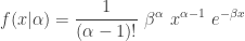
The following is the unconditional probability density function of
![\displaystyle \begin{aligned} f(x)&=\sum \limits_{\alpha=1}^\infty f(x \lvert \alpha) \ P[Y=\alpha] \\&=\sum \limits_{\alpha=1}^\infty \frac{1}{(\alpha-1)!} \ \beta^\alpha \ x^{\alpha-1} \ e^{-\beta x} \ p (1-p)^{\alpha-1} \\&=\beta p \ e^{-\beta x} \sum \limits_{\alpha=1}^\infty \frac{[\beta(1-p) x]^{\alpha-1}}{(\alpha-1)!} \\&=\beta p \ e^{-\beta x} \sum \limits_{\alpha=0}^\infty \frac{[\beta(1-p) x]^{\alpha}}{(\alpha)!} \\&=\beta p \ e^{-\beta x} \ e^{\beta(1-p) x} \end{aligned}](https://s0.wp.com/latex.php?latex=%5Cdisplaystyle+%5Cbegin%7Baligned%7D+f%28x%29%26%3D%5Csum+%5Climits_%7B%5Calpha%3D1%7D%5E%5Cinfty+f%28x+%5Clvert+%5Calpha%29+%5C+P%5BY%3D%5Calpha%5D+%5C%5C%26%3D%5Csum+%5Climits_%7B%5Calpha%3D1%7D%5E%5Cinfty+%5Cfrac%7B1%7D%7B%28%5Calpha-1%29%21%7D+%5C+%5Cbeta%5E%5Calpha+%5C+x%5E%7B%5Calpha-1%7D+%5C+e%5E%7B-%5Cbeta+x%7D+%5C+p+%281-p%29%5E%7B%5Calpha-1%7D+%5C%5C%26%3D%5Cbeta+p+%5C+e%5E%7B-%5Cbeta+x%7D+%5Csum+%5Climits_%7B%5Calpha%3D1%7D%5E%5Cinfty+%5Cfrac%7B%5B%5Cbeta%281-p%29+x%5D%5E%7B%5Calpha-1%7D%7D%7B%28%5Calpha-1%29%21%7D+%5C%5C%26%3D%5Cbeta+p+%5C+e%5E%7B-%5Cbeta+x%7D+%5Csum+%5Climits_%7B%5Calpha%3D0%7D%5E%5Cinfty+%5Cfrac%7B%5B%5Cbeta%281-p%29+x%5D%5E%7B%5Calpha%7D%7D%7B%28%5Calpha%29%21%7D+%5C%5C%26%3D%5Cbeta+p+%5C+e%5E%7B-%5Cbeta+x%7D+%5C+e%5E%7B%5Cbeta%281-p%29+x%7D+%5Cend%7Baligned%7D&bg=ffffff&fg=333333&s=0&c=20201002)
The above density function is that of an exponential distribution with rate parameter
Student t Distribution
Example 3 (discussed in the previous post) involves a normal distribution with a random mean. Example 8 involves a normal distribution with mean 0 and an uncertain variance, which follows a gamma distribution such that the two gamma parameters are related to a common parameter 
Example 8. Suppose that 

The following gives the ingredients of the normal-gamma mixture. The first item is the conditional density function of
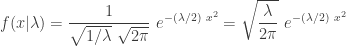

The following calculation derives the unconditional density function of
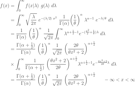
The above density function is in terms of the two parameters 

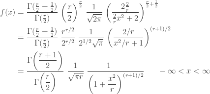
The above density function is that of a student t distribution with


Pingback: A catalog of parametric severity models | Topics in Actuarial Modeling
Pingback: Practice Problem Set 5 – Exercises for Severity Models « Practice Problems in Actuarial Modeling
Pingback: Several versions of negative binomial distribution « Practice Problems in Actuarial Modeling
Pingback: Gamma distribution and Poisson distribution | Applied Probability and Statistics
Pingback: Negative binomial distribution – A World of Ideas