
Mathematically, the Weibull distribution has a simple definition. It is mathematically tractable. It is also a versatile model. The Weibull distribution is widely used in life data analysis, particularly in reliability engineering. In addition to analysis of fatigue data, the Weibull distribution can also be applied to other engineering problems, e.g. for modeling the so called weakest link model.This post gives an introduction to the Weibull distribution.
_______________________________________________________________________________________________
Defining the Weibull Distribution
A random variable 
![\displaystyle f(y)=\frac{\tau}{\lambda} \ \biggl( \frac{y}{\lambda} \biggr)^{\tau-1} \text{exp} \biggl[- \biggl(\frac{y}{\lambda}\biggr)^\tau \ \biggr] \ \ \ ;y>0 \ \ \ \ \ \ \ \ \ \ \ \ \ \ \ \ \ \ \ \ \ \ \ \ \ \ \ \ \ \ (1)](https://s0.wp.com/latex.php?latex=%5Cdisplaystyle+f%28y%29%3D%5Cfrac%7B%5Ctau%7D%7B%5Clambda%7D+%5C+%5Cbiggl%28+%5Cfrac%7By%7D%7B%5Clambda%7D+%5Cbiggr%29%5E%7B%5Ctau-1%7D+%5Ctext%7Bexp%7D+%5Cbiggl%5B-+%5Cbiggl%28%5Cfrac%7By%7D%7B%5Clambda%7D%5Cbiggr%29%5E%5Ctau+%5C+%5Cbiggr%5D+%5C+%5C+%5C+%3By%3E0+%5C+%5C+%5C+%5C+%5C+%5C+%5C+%5C+%5C+%5C+%5C+%5C+%5C+%5C+%5C+%5C+%5C+%5C+%5C+%5C+%5C+%5C+%5C+%5C+%5C+%5C+%5C+%5C+%5C+%5C+%281%29&bg=ffffff&fg=333333&s=0&c=20201002)
where 

![\text{exp}[x]](https://s0.wp.com/latex.php?latex=%5Ctext%7Bexp%7D%5Bx%5D&bg=ffffff&fg=333333&s=0&c=20201002)


![\displaystyle F(y)=1- \text{exp} \biggl[- \biggl(\frac{y}{\lambda}\biggr)^\tau \ \biggr] \ \ \ \ \ \ \ \ \ \ \ \ \ \ \ \ \ \ \ \ \ \ \ \ \ \ \ \ \ \ \ \ \ \ \ \ \ \ \ \ \ \ \ \ \ \ \ \ \ \ (2)](https://s0.wp.com/latex.php?latex=%5Cdisplaystyle+F%28y%29%3D1-+%5Ctext%7Bexp%7D+%5Cbiggl%5B-+%5Cbiggl%28%5Cfrac%7By%7D%7B%5Clambda%7D%5Cbiggr%29%5E%5Ctau+%5C+%5Cbiggr%5D+%5C+%5C+%5C+%5C+%5C+%5C+%5C+%5C+%5C+%5C+%5C+%5C+%5C+%5C+%5C+%5C+%5C+%5C+%5C+%5C+%5C+%5C+%5C+%5C+%5C+%5C+%5C+%5C+%5C+%5C+%5C+%5C+%5C+%5C+%5C+%5C+%5C+%5C+%5C+%5C+%5C+%5C+%5C+%5C+%5C+%5C+%5C+%5C+%5C+%5C+%282%29&bg=ffffff&fg=333333&s=0&c=20201002)
_______________________________________________________________________________________________
Connection with the Exponential Distribution
The Weibull distribution can also arise naturally from the random sampling of an exponential random variable. A better way to view Weibull is through the lens of exponential. Taking an observation from an exponential distribution and raising it to a positive power will result in a Weibull observation. Specifically, the random variable 


![\displaystyle \begin{aligned} P[Y \le y]&=P[X^{\frac{1}{\tau}} \le y] \\&=P[X \le y^{\tau}] \\&=1-e^{-\frac{y^{\tau}}{\lambda^\tau}} \\&=1-e^{-(\frac{y}{\lambda})^\tau} \end{aligned}](https://s0.wp.com/latex.php?latex=%5Cdisplaystyle+%5Cbegin%7Baligned%7D+P%5BY+%5Cle+y%5D%26%3DP%5BX%5E%7B%5Cfrac%7B1%7D%7B%5Ctau%7D%7D+%5Cle+y%5D+%5C%5C%26%3DP%5BX+%5Cle+y%5E%7B%5Ctau%7D%5D+%5C%5C%26%3D1-e%5E%7B-%5Cfrac%7By%5E%7B%5Ctau%7D%7D%7B%5Clambda%5E%5Ctau%7D%7D+%5C%5C%26%3D1-e%5E%7B-%28%5Cfrac%7By%7D%7B%5Clambda%7D%29%5E%5Ctau%7D++%5Cend%7Baligned%7D&bg=ffffff&fg=333333&s=0&c=20201002)
_______________________________________________________________________________________________
Basic Properties
The idea of the Weibull distribution as a power of an exponential distribution simplifies certain calculation on the Weibull distribution. For example, a raw moment of the Weibull distribution is simply another raw moment of the exponential distribution. For an exponential random variable 
![E[X^k]](https://s0.wp.com/latex.php?latex=E%5BX%5Ek%5D&bg=ffffff&fg=333333&s=0&c=20201002)
![\displaystyle E[X^k]=\left\{ \begin{array}{ll} \displaystyle \Gamma(1+k) \ \theta^k &\ k>-1 \\ \text{ } & \text{ } \\ \displaystyle k! \ \theta^k &\ k \text{ is a positive integer} \end{array} \right.](https://s0.wp.com/latex.php?latex=%5Cdisplaystyle++E%5BX%5Ek%5D%3D%5Cleft%5C%7B+%5Cbegin%7Barray%7D%7Bll%7D+++++++++++++++++++++%5Cdisplaystyle++%5CGamma%281%2Bk%29+%5C+%5Ctheta%5Ek+%26%5C+k%3E-1+%5C%5C+++++++++++%5Ctext%7B+%7D+%26+%5Ctext%7B+%7D+%5C%5C+++++++++++%5Cdisplaystyle++k%21+%5C+%5Ctheta%5Ek+%26%5C+k+%5Ctext%7B+is+a+positive+integer%7D+++++++++++%5Cend%7Barray%7D+%5Cright.&bg=ffffff&fg=333333&s=0&c=20201002)
where 
For the Weibull random variable 
![\displaystyle E[Y]=E[X^{\frac{1}{\tau}}]=\Gamma \biggl(1+\frac{1}{\tau} \biggr) \ \lambda \ \ \ \ \ \ \ \ \ \ \ \ \ \ \ \ \ \ \ \ \ \ \ \ \ \ \ \ \ \ \ \ \ \ \ \ \ \ \ \ \ \ \ \ \ \ \ \ \ \ (3)](https://s0.wp.com/latex.php?latex=%5Cdisplaystyle+E%5BY%5D%3DE%5BX%5E%7B%5Cfrac%7B1%7D%7B%5Ctau%7D%7D%5D%3D%5CGamma+%5Cbiggl%281%2B%5Cfrac%7B1%7D%7B%5Ctau%7D+%5Cbiggr%29+%5C+%5Clambda+%5C+%5C+%5C+%5C+%5C+%5C+%5C+%5C+%5C+%5C+%5C+%5C+%5C+%5C+%5C+%5C+%5C+%5C+%5C+%5C+%5C+%5C+%5C+%5C+%5C+%5C+%5C+%5C+%5C+%5C+%5C+%5C+%5C+%5C+%5C+%5C+%5C+%5C+%5C+%5C+%5C+%5C+%5C+%5C+%5C+%5C+%5C+%5C+%5C+%5C+%283%29&bg=ffffff&fg=333333&s=0&c=20201002)
![\displaystyle E[Y^k]=E[X^{\frac{k}{\tau}}]=\Gamma \biggl(1+\frac{k}{\tau} \biggr) \ \lambda^k \ \ \ \ \ \ \ \ \ \ \ \ \ \ \ \ \ \ \ \ \ \ \ \ \ \ \ \ \ \ \ \ \ \ \ \ \ \ \ \ \ \ \ \ \ \ \ (4)](https://s0.wp.com/latex.php?latex=%5Cdisplaystyle+E%5BY%5Ek%5D%3DE%5BX%5E%7B%5Cfrac%7Bk%7D%7B%5Ctau%7D%7D%5D%3D%5CGamma+%5Cbiggl%281%2B%5Cfrac%7Bk%7D%7B%5Ctau%7D+%5Cbiggr%29+%5C+%5Clambda%5Ek+%5C+%5C+%5C+%5C+%5C+%5C+%5C+%5C+%5C+%5C+%5C+%5C+%5C+%5C+%5C+%5C+%5C+%5C+%5C+%5C+%5C+%5C+%5C+%5C+%5C+%5C+%5C+%5C+%5C+%5C+%5C+%5C+%5C+%5C+%5C+%5C+%5C+%5C+%5C+%5C+%5C+%5C+%5C+%5C+%5C+%5C+%5C+%284%29&bg=ffffff&fg=333333&s=0&c=20201002)
With the moments established, several other distributional quantities that are based on moments can also be established. The following shows the variance, skewness and kurtosis.
![\displaystyle Var[Y]=E[Y^2]-E[Y]^2=\biggl[ \Gamma \biggl(1+\frac{2}{\tau} \biggr)-\Gamma \biggl(1+\frac{1}{\tau} \biggr)^2 \biggr] \ \lambda^2 \ \ \ \ \ \ \ \ \ \ \ \ \ (5)](https://s0.wp.com/latex.php?latex=%5Cdisplaystyle+Var%5BY%5D%3DE%5BY%5E2%5D-E%5BY%5D%5E2%3D%5Cbiggl%5B+%5CGamma+%5Cbiggl%281%2B%5Cfrac%7B2%7D%7B%5Ctau%7D+%5Cbiggr%29-%5CGamma+%5Cbiggl%281%2B%5Cfrac%7B1%7D%7B%5Ctau%7D+%5Cbiggr%29%5E2+%5Cbiggr%5D+%5C+%5Clambda%5E2+%5C+%5C+%5C+%5C+%5C+%5C+%5C+%5C+%5C+%5C+%5C+%5C+%5C+%285%29&bg=ffffff&fg=333333&s=0&c=20201002)
![\displaystyle \begin{aligned} \gamma_1&=\frac{E[(Y-\mu)^3}{\sigma^3} \\&=\frac{E[Y^3]-3 \ \mu \ E[Y^2]+2 \ \mu^3}{\sigma^3} \\&\displaystyle =\frac{\Gamma \biggl(1+\frac{3}{\tau} \biggr) \lambda^3-3 \ \mu \ \Gamma \biggl(1+\frac{2}{\tau} \biggr) \lambda^2+2 \ \mu^3}{(\sigma^2)^{\frac{3}{2}}} \ \ \ \ \ \ \ \ \ \ \ \ \ \ \ \ \ \ \ \ \ \ \ \ \ \ \ \ \ \ \ (6) \end{aligned}](https://s0.wp.com/latex.php?latex=%5Cdisplaystyle+%5Cbegin%7Baligned%7D+%5Cgamma_1%26%3D%5Cfrac%7BE%5B%28Y-%5Cmu%29%5E3%7D%7B%5Csigma%5E3%7D+%5C%5C%26%3D%5Cfrac%7BE%5BY%5E3%5D-3+%5C+%5Cmu+%5C+E%5BY%5E2%5D%2B2+%5C+%5Cmu%5E3%7D%7B%5Csigma%5E3%7D+%5C%5C%26%5Cdisplaystyle+%3D%5Cfrac%7B%5CGamma+%5Cbiggl%281%2B%5Cfrac%7B3%7D%7B%5Ctau%7D+%5Cbiggr%29+%5Clambda%5E3-3+%5C+%5Cmu+%5C+%5CGamma+%5Cbiggl%281%2B%5Cfrac%7B2%7D%7B%5Ctau%7D+%5Cbiggr%29+%5Clambda%5E2%2B2+%5C+%5Cmu%5E3%7D%7B%28%5Csigma%5E2%29%5E%7B%5Cfrac%7B3%7D%7B2%7D%7D%7D+%5C+%5C+%5C+%5C+%5C+%5C+%5C+%5C+%5C+%5C+%5C+%5C+%5C+%5C+%5C+%5C+%5C+%5C+%5C+%5C+%5C+%5C+%5C+%5C+%5C+%5C+%5C+%5C+%5C+%5C+%5C+%286%29+%5Cend%7Baligned%7D&bg=ffffff&fg=333333&s=0&c=20201002)
![\displaystyle \begin{aligned} \gamma_2&=\frac{E[(Y-\mu)^4}{\sigma^4} \\&=\frac{E[Y^4]-4 \ \mu \ E[Y^3]+6 \ \mu^2 \ E[Y^2]-3 \ \mu^4}{\sigma^4} \\&\displaystyle =\frac{\Gamma \biggl(1+\frac{4}{\tau} \biggr) \lambda^4-4 \ \mu \ \Gamma \biggl(1+\frac{3}{\tau} \biggr) \lambda^3+6 \ \mu^2 \ \Gamma \biggl(1+\frac{2}{\tau} \biggr) \lambda^2-3 \ \mu^4}{\sigma^4} \ \ \ \ \ (7) \end{aligned}](https://s0.wp.com/latex.php?latex=%5Cdisplaystyle+%5Cbegin%7Baligned%7D+%5Cgamma_2%26%3D%5Cfrac%7BE%5B%28Y-%5Cmu%29%5E4%7D%7B%5Csigma%5E4%7D+%5C%5C%26%3D%5Cfrac%7BE%5BY%5E4%5D-4+%5C+%5Cmu+%5C+E%5BY%5E3%5D%2B6+%5C+%5Cmu%5E2+%5C+E%5BY%5E2%5D-3+%5C+%5Cmu%5E4%7D%7B%5Csigma%5E4%7D+%5C%5C%26%5Cdisplaystyle+%3D%5Cfrac%7B%5CGamma+%5Cbiggl%281%2B%5Cfrac%7B4%7D%7B%5Ctau%7D+%5Cbiggr%29+%5Clambda%5E4-4+%5C+%5Cmu+%5C+%5CGamma+%5Cbiggl%281%2B%5Cfrac%7B3%7D%7B%5Ctau%7D+%5Cbiggr%29+%5Clambda%5E3%2B6+%5C+%5Cmu%5E2+%5C+%5CGamma+%5Cbiggl%281%2B%5Cfrac%7B2%7D%7B%5Ctau%7D+%5Cbiggr%29+%5Clambda%5E2-3+%5C+%5Cmu%5E4%7D%7B%5Csigma%5E4%7D+%5C+%5C+%5C+%5C+%5C+%287%29+%5Cend%7Baligned%7D&bg=ffffff&fg=333333&s=0&c=20201002)
The notation 


Another calculation that is easily accessible for the Weibull distribution is that of the percentiles. It is easy to solve for 

Another basic and important property to examine is the failure rate. The failure rate of a distribution is the ratio of the density function to its survival function. The following is the failure of the Weibull distribution.

See here for a discussion of the failure rate in conjunction with the exponential distribution. Suppose that the distribution in question is a lifetime distribution (time until termination or death). Then the failure rate 

_______________________________________________________________________________________________
When the Parameters Vary
The discussion in the previous section might give the impression that all Weibull distributions (when the parameters vary) behave in the same way. We now look at examples showing that as 
Example 1
The following diagram shows the PDFs of the Weibull distribution with 


Figure 1
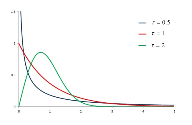
Figure 1 shows the effect of the shape parameter taking on different values while keeping the scale parameter fixed. The effect is very pronounced on the skewness. All three density curves are right skewed. The PDF with 


Another clear effect of the shape parameter is the thickness of the tail (in this case the right tail). Figure 1 suggests that the PDF with 
![\displaystyle \begin{array}{lllllll} \text{ } &\text{ } & \tau=0.5 & \text{ } & \tau=1 & \text{ } & \tau=2 \\ \text{ } & \text{ } &\text{Blue Curve} & \text{ } & \text{Red Curve} & \text{ }& \text{Green Curve} \\ \text{ } & \text{ } & \text{ } & \text{ } & \text{ } \\ P[X>2] &\text{ } & 0.2431 & \text{ } & 0.1353 & \text{ } & 0.0183\\ \text{ } & \text{ } & \text{ } & \text{ } & \text{ } \\ P[X>3] &\text{ } & 0.1769 & \text{ } & 0.0498 & \text{ } & 0.0003355 \\ \text{ } & \text{ } & \text{ } & \text{ } & \text{ } \\ P[X>4] &\text{ } & 0.1353 & \text{ } & 0.0183 & \text{ } & \displaystyle 1.125 \times 10^{-7} \\ \text{ } & \text{ } & \text{ } & \text{ } & \text{ } \\ P[X>5] &\text{ } & 0.1069 & \text{ } & 0.00674 & \text{ } & 1.389 \times 10^{-11} \\ \text{ } & \text{ } & \text{ } & \text{ } & \text{ } \\ P[X>10] &\text{ } & 0.0423 & \text{ } & 0.0000454 & \text{ } & 3.72 \times 10^{-44} \\ \text{ } & \text{ } & \text{ } & \text{ } & \text{ } \\ P[X>25] &\text{ } & 0.00673 & \text{ } & 1.39 \times 10^{-11} & \text{ } & 3.68 \times 10^{-272} \end{array}](https://s0.wp.com/latex.php?latex=%5Cdisplaystyle+%5Cbegin%7Barray%7D%7Blllllll%7D+%5Ctext%7B+%7D+%26%5Ctext%7B+%7D+%26+%5Ctau%3D0.5++%26+%5Ctext%7B+%7D+%26+%5Ctau%3D1+%26+%5Ctext%7B+%7D+%26+%5Ctau%3D2++%5C%5C++%5Ctext%7B+%7D+%26+%5Ctext%7B+%7D+%26%5Ctext%7BBlue+Curve%7D+%26+%5Ctext%7B+%7D+%26+%5Ctext%7BRed+Curve%7D+%26+%5Ctext%7B+%7D%26+%5Ctext%7BGreen+Curve%7D+%5C%5C++%5Ctext%7B+%7D+%26+%5Ctext%7B+%7D+%26+%5Ctext%7B+%7D+%26+%5Ctext%7B+%7D+%26+%5Ctext%7B+%7D+%5C%5C++P%5BX%3E2%5D+%26%5Ctext%7B+%7D+%26+0.2431+%26+%5Ctext%7B+%7D+%26+0.1353++%26+%5Ctext%7B+%7D+%26+0.0183%5C%5C+++++%5Ctext%7B+%7D+%26+%5Ctext%7B+%7D+%26+%5Ctext%7B+%7D+%26+%5Ctext%7B+%7D+%26+%5Ctext%7B+%7D+%5C%5C++P%5BX%3E3%5D+%26%5Ctext%7B+%7D+%26+0.1769+%26+%5Ctext%7B+%7D+%26+0.0498+%26+%5Ctext%7B+%7D+%26+0.0003355+%5C%5C++%5Ctext%7B+%7D+%26+%5Ctext%7B+%7D+%26+%5Ctext%7B+%7D+%26+%5Ctext%7B+%7D+%26+%5Ctext%7B+%7D+%5C%5C++P%5BX%3E4%5D+%26%5Ctext%7B+%7D+%26+0.1353+%26+%5Ctext%7B+%7D+%26+0.0183+%26+%5Ctext%7B+%7D+%26+%5Cdisplaystyle+1.125+%5Ctimes+10%5E%7B-7%7D+%5C%5C++%5Ctext%7B+%7D+%26+%5Ctext%7B+%7D+%26+%5Ctext%7B+%7D+%26+%5Ctext%7B+%7D+%26+%5Ctext%7B+%7D+%5C%5C++P%5BX%3E5%5D+%26%5Ctext%7B+%7D+%26+0.1069+%26+%5Ctext%7B+%7D+%26+0.00674+%26+%5Ctext%7B+%7D+%26+1.389+%5Ctimes+10%5E%7B-11%7D+%5C%5C++%5Ctext%7B+%7D+%26+%5Ctext%7B+%7D+%26+%5Ctext%7B+%7D+%26+%5Ctext%7B+%7D+%26+%5Ctext%7B+%7D+%5C%5C++P%5BX%3E10%5D+%26%5Ctext%7B+%7D+%26+0.0423+%26+%5Ctext%7B+%7D+%26+0.0000454+%26+%5Ctext%7B+%7D+%26+3.72+%5Ctimes+10%5E%7B-44%7D+%5C%5C++%5Ctext%7B+%7D+%26+%5Ctext%7B+%7D+%26+%5Ctext%7B+%7D+%26+%5Ctext%7B+%7D+%26+%5Ctext%7B+%7D+%5C%5C++P%5BX%3E25%5D+%26%5Ctext%7B+%7D+%26+0.00673+%26+%5Ctext%7B+%7D+%26+1.39+%5Ctimes+10%5E%7B-11%7D+%26+%5Ctext%7B+%7D+%26+3.68+%5Ctimes+10%5E%7B-272%7D++%5Cend%7Barray%7D&bg=ffffff&fg=333333&s=0&c=20201002)
It is clear from the above table that the Weibull distribution with the blue curve assigns more probabilities to the higher values. The mean of the distribution for blue curve is 2. The right tail 


Let’s compare the density curves in Figure 1 with their failure rates. The following figure shows the failure rates for these three Weibull distributions.
Figure 2
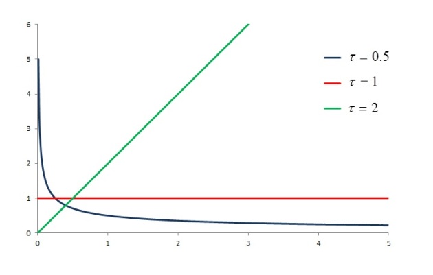
According to the definition in 


The blue curve in Figure 1 (

Example 2
We now compare Weibull distributions with various values for 
Figure 3
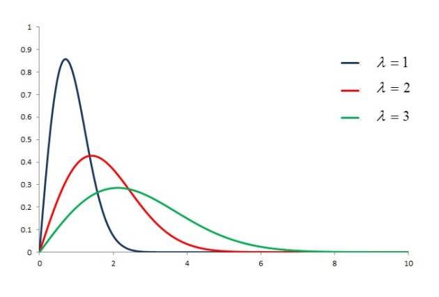
The effect of the scale parameter 

The next example is a computational exercise.
Example 3
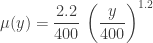
The time until failure (in months) of a semiconductor device has a Weibull distribution with shape parameter 

- Give the density function and the survival function.
- Determine the probability that the device will last at least 500 hours.
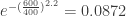
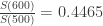
- Determine the probability that the device will last at least 600 hours given that it has been running for over 500 hours.
- Find the mean and standard deviation of the time until failure.
- Determine the failure rate function of the Weibull time until failure.
To obtain the density function, the survival function and the failure rate, follow the relationships in 
![\displaystyle f(y)=\frac{2.2}{400} \ \biggl( \frac{y}{400} \biggr)^{1.2} \text{exp} \biggl[- \biggl(\frac{y}{400}\biggr)^{2.2} \ \biggr]](https://s0.wp.com/latex.php?latex=%5Cdisplaystyle+f%28y%29%3D%5Cfrac%7B2.2%7D%7B400%7D+%5C+%5Cbiggl%28+%5Cfrac%7By%7D%7B400%7D+%5Cbiggr%29%5E%7B1.2%7D+%5Ctext%7Bexp%7D+%5Cbiggl%5B-+%5Cbiggl%28%5Cfrac%7By%7D%7B400%7D%5Cbiggr%29%5E%7B2.2%7D+%5C+%5Cbiggr%5D&bg=ffffff&fg=333333&s=0&c=20201002)
![\displaystyle S(y)=\text{exp} \biggl[- \biggl(\frac{y}{400}\biggr)^{2.2} \biggr]](https://s0.wp.com/latex.php?latex=%5Cdisplaystyle+S%28y%29%3D%5Ctext%7Bexp%7D+%5Cbiggl%5B-+%5Cbiggl%28%5Cfrac%7By%7D%7B400%7D%5Cbiggr%29%5E%7B2.2%7D+%5Cbiggr%5D&bg=ffffff&fg=333333&s=0&c=20201002)
Note that the Weibull failure rate is the ratio of the density function to the survival function. In this case, the failure is an increasing function of
The probability that the device will last over 500 hours is 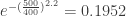
To find the mean and variance, we need to evaluate the gamma function. Using Excel, we obtain the following two values of the gamma function (as shown here):


The mean and standard deviation of the time until failure are:
![E[Y]=\Gamma(1+\frac{1}{2.2}) \times 400=354.2499042](https://s0.wp.com/latex.php?latex=E%5BY%5D%3D%5CGamma%281%2B%5Cfrac%7B1%7D%7B2.2%7D%29+%5Ctimes+400%3D354.2499042&bg=ffffff&fg=333333&s=0&c=20201002)
![E[Y^2]=\Gamma(1+\frac{2}{2.2}) \times 400^2=154385.9982](https://s0.wp.com/latex.php?latex=E%5BY%5E2%5D%3D%5CGamma%281%2B%5Cfrac%7B2%7D%7B2.2%7D%29+%5Ctimes+400%5E2%3D154385.9982&bg=ffffff&fg=333333&s=0&c=20201002)
![Var[Y]=E[Y^2]-E[Y]^2=28893.00363](https://s0.wp.com/latex.php?latex=Var%5BY%5D%3DE%5BY%5E2%5D-E%5BY%5D%5E2%3D28893.00363&bg=ffffff&fg=333333&s=0&c=20201002)
![\sigma_Y=\sqrt{Var[Y]}=169.9794212](https://s0.wp.com/latex.php?latex=%5Csigma_Y%3D%5Csqrt%7BVar%5BY%5D%7D%3D169.9794212&bg=ffffff&fg=333333&s=0&c=20201002)
_______________________________________________________________________________________________
The Weibull Failure Rates
Looking at the failure rate function indicated in 
When the shape parameter
In some applications, it may be necessary to model each phase of a lifetime separately, e.g. the early phase with a Weibull distribution with
Figure 4
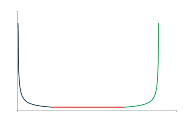
The blue part of the bathtub curve is the early phase of the lifetime, which is characterized by decreasing failure rate. This is the early-life period in which the defective products die off and are taken out of the study. The next period is the useful-life period, the red part of the curve, in which the failures are random that are independent of age. In this phase, the failure rate is constant or near constant. The green part of the bathtub curve is characterized by increasing failure rates, which is the wear-out phase of the lifetime being studied.
_______________________________________________________________________________________________
Weakest Link Model
Another attractiveness of the Weibull model is that it can be used to model the so called the weakest link model. Consider a machine or device that has multiple components. Suppose that the device dies or fails when any one of the components fails. The lifetime of such a machine or device is the time to the first failure. Such a lifetime model is called the weakest link model. It can be shown that under these conditions a Weibull distribution is a good model for the distribution of the lifetime of such a machine or device.
If the time until failure of the individual components are indpendent and identically distributed Weibull random variables, then it follows that the minimum of of the Weibull random variables is also a Weibull random variable. To see this, let 

![\displaystyle \begin{aligned} P[Y >y]&=P[\text{all } X_i >y] \\&=\biggl(e^{-(\frac{y}{\lambda})^\tau} \biggr)^n \\&=e^{-n (\frac{y}{\lambda})^\tau} \\&=e^{-(\frac{y}{\lambda_1})^\tau} \end{aligned}](https://s0.wp.com/latex.php?latex=%5Cdisplaystyle+%5Cbegin%7Baligned%7D+P%5BY+%3Ey%5D%26%3DP%5B%5Ctext%7Ball+%7D+X_i+%3Ey%5D++%5C%5C%26%3D%5Cbiggl%28e%5E%7B-%28%5Cfrac%7By%7D%7B%5Clambda%7D%29%5E%5Ctau%7D+%5Cbiggr%29%5En+%5C%5C%26%3De%5E%7B-n+%28%5Cfrac%7By%7D%7B%5Clambda%7D%29%5E%5Ctau%7D+%5C%5C%26%3De%5E%7B-%28%5Cfrac%7By%7D%7B%5Clambda_1%7D%29%5E%5Ctau%7D++%5Cend%7Baligned%7D&bg=ffffff&fg=333333&s=0&c=20201002)
where 


_______________________________________________________________________________________________
The Moment Generating Function
The post is concluded with a comment on the moment generating function for the Weibull distribution. Note that relationship 


To see this, start with the power series for 

![\displaystyle M(t)=E[e^{t X}]=\sum \limits_{n=0}^\infty \ \frac{t^n}{n!} \ E[X^n]](https://s0.wp.com/latex.php?latex=%5Cdisplaystyle+M%28t%29%3DE%5Be%5E%7Bt+X%7D%5D%3D%5Csum+%5Climits_%7Bn%3D0%7D%5E%5Cinfty+%5C+%5Cfrac%7Bt%5En%7D%7Bn%21%7D+%5C+E%5BX%5En%5D&bg=ffffff&fg=333333&s=0&c=20201002)
Since the positive moments exist for the Weibull distribution, the higher moments from
When 

_______________________________________________________________________________________________
Further Information
Further information can be found here and here.
_______________________________________________________________________________________________


Pingback: More topics on the exponential distribution | Topics in Actuarial Modeling
Hi! could i have matlab scripts for this topic?
LikeLike
Pingback: Transformed exponential distributions | Topics in Actuarial Modeling
Pingback: Examples of mixtures | Topics in Actuarial Modeling
Pingback: Pareto Type I versus Pareto Type II « Practice Problems in Actuarial Modeling
Pingback: A catalog of parametric severity models | Topics in Actuarial Modeling
Pingback: Practice Problem Set 5 – Exercises for Severity Models « Practice Problems in Actuarial Modeling
Pingback: Transformation of univariate random variables | Probability and Statistics Problem Solve